System Identification Using Multilayer Differential Neural Networks: A New Result
Abstract
In previous works, a learning law with a dead zone function was developed for multilayer differential neural networks. This scheme requires strictly a priori knowledge of an upper bound for the unmodeled dynamics. In this paper, the learning law is modified in such a way that this condition is relaxed. By this modification, the tuning process is simpler and the dead-zone function is not required anymore. On the basis of this modification and by using a Lyapunov-like analysis, a stronger result is here demonstrated: the exponential convergence of the identification error to a bounded zone. Besides, a value for upper bound of such zone is provided. The workability of this approach is tested by a simulation example.
1. Introduction
During the last four decades system identification has emerged as a powerful and effective alternative to the first principles modeling [1–4]. By using the first approach, a satisfactory mathematical model of a system can be obtained directly from an input and output experimental data set [5]. Ideally no a priori knowledge of the system is necessary since this is considered as a black box. Thus, the time employed to develop such model is reduced significantly with respect to a first principles approach. For the linear case, system identification is a problem well understood and enjoys well-established solutions [6]. However, the nonlinear case is much more challenging. Although some proposals have been presented [7], the class of considered nonlinear systems can result very limited. Due to their capability of handling a more general class of systems and due to advantages such as the fact of not requiring linear in parameters and persistence of excitation assumptions [8], artificial neural networks (ANNs) have been extensively used in identification of nonlinear systems [9–12]. Their success is based on their capability of providing arbitrarily good approximations to any smooth function [13–15] as well as their massive parallelism and very fast adaptability [16, 17].
An artificial neural network can be simply considered as a nonlinear generic mathematical formula whose parameters are adjusted in order to represent the behavior of a static or dynamic system [18]. These parameters are called weights. Generally speaking, ANN can be classified as feedforward (static) ones, based on the back propagation technique [19] or as recurrent (dynamic) ones [17]. In the first network type, system dynamics is approximated by a static mapping. These networks have two major disadvantages: a slow learning rate and a high sensitivity to training data. The second approach (recurrent ANN) incorporates feedback into its structure. Due to this feature, recurrent neural networks can overcome many problems associated with static ANN, such as global extrema search, and consequently have better approximation properties. Depending on their structure, recurrent neural networks can be classified as discrete-time ones or differential ones.
2. Multilayer Neural Identifier
The problem of identifying system (2.1) based on the multilayer differential neural network (2.2) consists of, given the measurable state xt and the input ut, adjusting on line the weights W1,t, W2,t, V1,t, and V2,t by proper learning laws such that the identification error can be reduced.
- (A1)
System (2.1) satisfies the (uniform on t) Lipschitz condition, that is,
- (A2)
The differences of functions σ(·) and ϕ(·) fulfil the generalized Lipschitz conditions
(2.6)where(2.7)Λ1 ∈ ℜm×m, Λ2 ∈ ℜr×r, Λσ ∈ ℜn×n, Λϕ ∈ ℜn×n are known positive definite matrices, and are constant matrices which can be selected by the designer.As σ(·) and ϕ(·) fulfil the Lipschitz conditions and from Lemma A.1 proven in [26] the following is true:
(2.8)(2.9)where(2.10)νσ ∈ ℜm and νiϕ ∈ ℜn are unknown vectors but bounded by , , respectively; , , l1 and l2 are positive constants which can be defined as , , where Lg,1 and Lg,2 are global Lipschitz constants for σ(·) and ϕi(·), respectively. - (A3)
The nonlinear function γ(·) is such that where is a known positive constant.
- (A4)
Unmodeled dynamics is bounded by
(2.11)where and are known positive constants and Λ3 ∈ ℜn×n is a known positive definite matrix and can be defined as and are constant matrices which can be selected by the designer. - (A5)
The deterministic disturbance is bounded, that is, , Λ4 is a known positive definite matrix.
- (A6)
The following matrix Riccati equation has a unique, positive definite solution P:
(2.12)where(2.13)Q0 is a positive definite matrix which can be selected by the designer.
Remark 2.1. Based on [30, 31], it can be established that the matrix Riccati equation (2.12) has a unique positive definite solution P if the following conditions are satisfied;
- (a)
The pair (A, R1/2) is controllable, and the pair (Q1/2, A) is observable.
- (b)
The following matrix inequality is fulfilled:
(2.14)Both conditions can relatively easily be fulfilled if A is selected as a stable diagonal matrix.
- (A7)
It exists a bounded control ut, such that the closed-loop system is quadratic stable, that is, it exists a Lyapunov function V0 > 0 and a positive constant λ such that
(2.15)Additionally, the inequality must be satisfied.
Theorem 2.2. If the assumptions (A1)–(A7) are satisfied and the weight matrices W1,t, W2,tV1,t, and V2,t of the neural network (2.2) are adjusted by the learning law (2.16), then
- (a)
the identification error and the weights are bounded:
(2.18) - (b)
the identification error Δt satisfies the following tracking performance:
3. Exponential Convergence of the Identification Process
- (B4)
In a compact set Ω ∈ ℜn, unmodeled dynamics is bounded by where is a constant not necessarily a priori known.
Remark 3.1. (B4) is a common assumption in the neural network literature [17, 22]. As mentioned in Section 2, is given by . Note that and are bounded functions because σ(·) and ϕ(·) are sigmoidal functions. As xt belongs to Ω, clearly xt is also bounded. Therefore, assumption B4 implies implicitly that f(xt, ut, t) is a bounded function in a compact set Ω ∈ ℜn.
Although certainly assumption (B4) is more restrictive than assumption (A4), from now on, assumption (A7) is not needed anymore.
Theorem 3.2. If the assumptions (A1)–(A3), (B4), (A5)-(A6) are satisfied and the weight matrices W1,t, W2,t, V1,t, and V2,t of the neural network (2.2) are adjusted by the learning law (3.1), then
- (a)
the identification error and the weights are bounded:
(3.2) - (b)
the norm of identification error converges exponentially to a region bounded given by
Proof of Theorem 3.2. Before beginning analysis, the dynamics of the identification error Δt must be determined. The first derivative of Δt is
Remark 3.3. Based on the results presented in [32, 33], and, from the inequality (3.38), uniform stability for the identification error can be guaranteed.
Remark 3.4. Although, in [34], the asymptotic convergence of the identification error to zero is proven for multilayer neural networks, the considered class of nonlinear systems is much more restrictive than in this work.
4. Tuning of the Multilayer Identifier
In this section, some details about the selection of the parameters for the neural identifier are presented. In first place, it is important to mention that the positive definite matrices Λ1 ∈ ℜm×m, Λ2 ∈ ℜr×r, Λσ ∈ ℜn×n, Λϕ ∈ ℜn×n, Λ3 ∈ ℜn×n, and Λ4 ∈ ℜn×n presented throughout assumptions (A2)–(A5) are known a priori. In fact, their selection can be very free. Although, in many cases, identity matrices can be enough, the corresponding freedom of selection can be used to satisfy the conditions specified in Remark 2.1.
Other important design decision is related to the proper number of elements m or neurons for σ(·). A good point of departure is to select m = n where n is the dimension of the state vector xt. Normally, this selection is enough in order to produce adequate results. In other case, m should be selected such as m > n. With respect to ϕ(·), for simplicity, a first attempt could be to set the elements of this matrix as zeroes except for the main diagonal.
Another very important question which must be taken into account is the following: how should the weights be selected? Ideally, these weights should be chosen in such a way that the modelling error or unmodeled dynamics can be minimized. Likewise, the design process must consider the solution of the Riccati equation (2.12). In order to guarantee the existence of a unique positive definite solution P for (2.12), the conditions specified in Remark 2.1 must be satisfied. However, these conditions could not be fulfilled for the optimal weights. Consequently, different values for and could be tested until a solution for (2.12) can be found. At the same time, the designer should be aware of that as take values increasingly different from the optimal ones, the upper bound for unmodeled dynamics in assumption B4 becomes greater. With respect to the initial values for W1,t, W2,t, V1,t, and V2,t, some authors, for example [26], simply select , and .
Finally, a last recommendation, in order to achieve a proper performance of the neural network, the variables in the identification process should be normalized. In this context, normalization means to divide each variable by its corresponding maximum value.
5. Numerical Example
In this section, a very simple but illustrative example is presented in order to clarify the tuning process of the neural identifier and compare the advantages of the scheme developed in this paper with respect to the results of previous works [26–29].
For simplicity, ξt is assumed equal to zero. It is very important to note that (5.1) is only used as a data generator since apart from the assumptions (A1)–(A3), (B4), (A5)-(A6), none previous knowledge about the unknown system (5.1) is required to satisfactorily carry out the identification process.
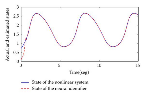
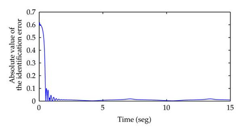
The results of the identification process are displayed in Figures 1 and 2. In Figure 1, the state xt of the nonlinear system (5.1) is represented by solid line whereas the state is represented by dashed line. Both states were obtained by using Simulink with the numerical method ode23s. In order to appreciate better the quality of the identification process, the absolute value of the identification error is showed in Figure 2. Clearly, the new learning laws proposed in this paper exhibit a satisfactory behavior.


Now, which is the practical advantage of this method with respect to previous works [26–29]? The determination of and more still (parameters associated with assumption A.4) can result difficult. Besides, assuming that is equal to zero, can result excessively large inclusive for simple systems. For example, for system (5.1) and the values selected for the parameters of the identifier, can approximately be estimated as 140. This implies that the learning laws (2.16) are activated only when |Δt| ≥ 70 due to the dead-zone function st. Thus, although the results presented in works [26–29] are technically right, on these conditions, that is, , the performance of the identifier results completely unsatisfactory from a practical point of view since the corresponding identification error is very high. To avoid this situation, it is necessary to be very careful with the selection of weights , and in order to minimize the unmodeled dynamics . However, with these optimal weights, the matrix Riccati equation could have no solution. This dilemma is overcome by means of the learning laws (3.1) developed in this paper. In fact, as can be appreciated, a priory knowledge of is not required anymore for the proper implementation of (3.1).
6. Conclusions
In this paper, a modification of a learning law for multilayer differential neural networks is proposed. By this modification, the dead-zone function is not required anymore and a stronger result is here guaranteed: the exponential convergence of the identification error norm to a bounded zone. This result is thoroughly proven. First, the dynamics of the identification error is determined. Next, a proper nonnegative function is proposed. A bound for the first derivative of such function is established. This bound is formed by the negative of the original nonnegative function multiplied by a constant parameter α plus a constant term. Thus, the convergence of the identification error to a bounded zone can be guaranteed. Apart from the theoretical importance of this result, from a practical point of view, the learning law here proposed is easier to implement and tune. A numerical example confirms the efficiency of this approach.
Acknowledgments
The authors would like to thank the anonymous reviewers for their helpful comments and advice which contributed to improve this paper. First author would like to thank the financial support through a postdoctoral fellowship from Mexican National Council for Science and Technology (CONACYT).


