Stochastic Functional Differential Equation under Regime Switching

Assumption A. For each integer k ≥ 1, …, there is a positive number H_k such that

for all t ≥ 0 and those φ₁, φ₂ ∈ C([−τ, 0]; Rⁿ) with ∥φ₁∥∨∥φ₂∥≤k.

Throughout this paper, unless otherwise specified, we let (Ω, ℱ, {ℱ_t} _t≥0, P) be a complete probability space with a filtration {ℱ_t} _t≥0 satisfying the usual conditions (i.e., it is right continuous and ℱ₀ contains all P-null sets). Let W_i(t) (i = 1,2), t ≥ 0, be the standard Brownian motion defined on this probability space. We also denote by $$. Let r(t) be a right-continuous Markov chain on the probability space taking values in a finite state space 𝕊 = {1,2, …, N} with the generator $$ given by

where δ > 0. Here γ_uv is the transition rate from u to v and γ_uv ≥ 0 if u ≠ v while We assume that the Markov chain r(·) is independent on the Brownian motion W_i(·), i = 1,2; furthermore, W₁ and W₂ are independent.

In addition, throughout this paper, let $$ denote the family of all positive real-valued functions V(x, t, k) on Rⁿ × [−τ, ∞) × 𝕊 which are continuously twice differentiable in x and once in t. If for the following equation

there exists V ∈ C^2,1(Rⁿ × [−τ, ∞) × 𝕊; R₊), define an operator ℓV from C([−τ, 0]; Rⁿ) × R₊ × 𝕊 to R by where Here we should emphasize that [1, Page 305] the operator ℓV (thought as a single notation rather than ℓ acting on V) is defined on C([−τ, 0]; Rⁿ) × R₊ × 𝕊 although V is defined on Rⁿ × [−τ, ∞) × 𝕊.

Assumption B. For each i ∈ 𝕊, there exist nonnegative constants $$ and probability measures μ, on [−τ, 0] such that

for any φ ∈ C([−τ, 0]; Rⁿ).

Theorem 2.1. Under the conditions of Assumptions A and B, if 2β > α, and σ(i) ≠ 0 for i = 1,2, …, n, there almost surely exists a unique globally solution x(t) to (1.1) on t ≥ −τ for any given initial data φ ∈ C([−τ, 0]; Rⁿ).

Proof. Since the coefficients of (1.1) are locally Lipschitz, there is a unique maximal local solution x(t) on t ∈ [−τ, τ_e), where τ_e is the explosion time. In order to prove this solution is global, we need to show that τ_e = ∞ a.s. Let m₀ > 0 be sufficiently large such that 1/m₀ < min _{−τ≤θ≤0} |ξ(θ)| < max _{−τ≤θ≤0} |ξ(θ)| < m₀. For each m ≥ m₀, we define the stopping time

Clearly τ_m is increasing as m → ∞. Set τ_∞ = lim _m→∞τ_m, if we can obtain that τ_∞ = ∞ a.s., then τ_e = ∞ a.s. for all t ≥ 0. That is, to complete the proof, also equivalent to prove that, for any t > 0, P(τ_m ≤ t) → 0 as m → ∞. If this conclusion is false, there is a pair of constants T > 0 and ɛ ∈ (0,1) such that So there exists an integer m₁ ≥ m₀ such that

To prove the conclusion that we desired, for any p ∈ (0,1/2), define a C²-function: $$ by

where {c(k), 1 ≤ k ≤ N} is positive constant sequence. Applying the generalized Itô formula, where ℓV is computed as

Let $$. For any k, l ∈ 𝕊, we get

Therefore,

According to Assumption B, the first term in (2.7)

By the Young inequality and noting that p ∈ (0,1/2), it is obvious that

where the first inequality we have used the elementary inequality: for any a, b ≥ 0 and r ∈ (0,1), (a+b)^r ≤ a^r + b^r. Therefore we have where Using the elementary inequality: for any a, b ≥ 0 and r ≥ 1, (a + b) ^r ≤ 2^r−1(a^r + b^r), we obtain that $$, also we have Therefore, Noting that p ∈ (0,1/2) and 2β > α ≥ 0, by the boundedness property of polynomial functions, there exists a positive constant M_k such that $$. Taking expectation from two sides of (2.6) leads to and from (2.12) and (2.15), we have where we denote $$.

By the Fubini theorem and a substitution technique, we may compute that

Similarly, Therefore we rewrite (2.17) into where K_T is bounded and K_T is independent of m.

By the definition of τ_m, x(τ_m) = m or 1/m, so let Ω_m = {τ_m ≤ T} for m ≥ m₁ and by (2.6), noting that for every ω ∈ Ω_m, there is some m such that x_m(τ_m, ω) equals either m or 1/m hence

Letting m → ∞ implies that So we must obtain τ_∞ = ∞ a.s., as required. The proof is complete.

Lemma 3.1. Under the conditions of Theorem 2.1, for any p ∈ (0,1/2), there exists a constant K_p independent on the initial data such that the global solution x(t) of SDE (1.1) has the property that

Proof. First, Theorem 2.1 indicates that the solution x(t) of (1.1) almost surely remain in Rⁿ for all t ≥ −τ with probability 1.

Applying the Itô formula to e^ɛtV(x, k) and taking expectation yields

Here ℓV(φ, k) is defined as before (2.7).

Now we consider the function

Similar to the proof of Theorem 2.1, then we know (3.3) is upper bounded; there exists constant ψ_k such that Φ_k(x)≤(1 + |x|²) ^2−pΦ_k(x) ≤ ψ_k ≤ Ψ : = max _1≤k≤N ψ_k; therefore, (3.2) implies that

We have the following calculus transformation:

Similarly,

We therefore have from (3.4)

Clearly,

denote $$; therefore, which yields This means that the solution is bounded in the 2pth moment; the stochastically ultimate boundedness will follow directly.

Definition 3.2. The solutions x(t) of SDE (1.1) are called stochastically ultimately bounded, if for any ϵ ∈ (0,1), there is a positive constant χ( = χ(ϵ)), such that the solution of SDE (1.1) with any positive initial value has the property that

Theorem 3.3. The solution of (1.1) is stochastically ultimately bounded under the condition Lemma 3.1; that is, for any ϵ ∈ (0,1), there is a positive constant χ( = χ(ϵ)), such that for any positive initial value the solution of Lemma 3.1 has the property that

Proof. This can be easily verified by Chebyshev′s inequality and Lemma 3.1 by choosing $$ sufficiently large because of the following

Assumption C. For each i ∈ 𝕊, there exist nonnegative constants $$ and probability measures μ, on [−τ, 0] such that

for any φ ∈ C([−τ, 0]; Rⁿ).

Clearly, Assumption C is stronger than the one-sided polynomial growth condition Assumption B. Therefore, Theorems 2.1 and Lemma 3.1 still hold under Assumption C.

In [10, Page 165], for a given nonlinear SDE with Markovian switching

any solution starting form a nonzero state will remain to be non-zero. But for the system (1.1) the drift coefficient is a functional, so we will prove this non-zero property under Assumption C.

Lemma 4.1. Let x(t) be the global solution of (1.1). Under Assumption C, if 2β > α and σ(i) ≠ 0, for any non-zero initial data x(0) ≠ 0

that is, almost all the sample path of any solution starting from a non-zero state will never reach the origin.

Proof. For any initial data ξ ∈ C([−τ, 0]; Rⁿ) satisfying x(0) ≠ 0, for sufficiently large positive number i₀, such that |x(0)| > 1/i₀. For each integer i ≥ i₀, define the stopping time

Clearly, ρ_i is increasing as i → ∞ and ρ_i → ρ_∞ a.s. If we can show that ρ_∞ = ∞ a.s., the desired result P(x(t) ≠ 0) = 1 on t ≥ 0 follows. This is equivalent to proving that, for any t > 0, P(ρ_i ≤ t) → 0 as i → ∞.

To prove this statement, define a C²-function

where V₁(·) > 0 and V₁(0⁺) = ∞. Applying the Itô formula and taking the expectation yield where ℓV₁ is defined as for any φ ∈ C([−τ, 0]; Rⁿ). By Assumption C and the Young inequality, the first term of (4.8) will be written as Substituting (4.9) into (4.8) gives where Noting (2.9) and 2β > α, σ(k) ≠ 0, using the boundedness property of polynomial functions, there exists a constant $$ such that $$.

Furthermore, we may estimate that

It therefore follows that

We know that

which implies that as required. The proof is completed.

Theorem 4.2. Suppose the Markov chain r(t) is irreducible, under Assumption A and C, if for δ ∈ (0,1), k ∈ 𝕊, σ(k) ≠ 0 and 2β > α, the solution x(t) of SDE (1.1) with any initial data ξ ∈ C([−τ, 0]; Rⁿ) satisfying x(0) ≠ 0 has the property

where In particular, the nonlinear hybrid system (1.1) is almost surely exponentially stable if

Proof. By Theorem 2.1 and Lemma 4.1, (1.1) almost surely admits a global solution x(t) for all t ≥ 0 and x(t) ≠ 0 almost surely. Applying the Itô formula to the function log  | x(t)| leads to

Define $$; clearly M(t) is a continuous local martingale with the quadratic variation For any δ ∈ (0,1), choose ϑ > 0 such that δϑ > 1 and each positive integer n > 0; the exponential martingale inequality yields

Since $$, by the Borel-Cantelli lemma, there exists an Ω₀ ⊂ Ω with ℙ(Ω₀) = 1 such that for any ω ∈ Ω₀, there exists an integer n(ω), when n > n(ω) and n − 1 ≤ t ≤ n,

This, together with Assumption C, denote $$ and $$; noting the definition of (4.17), we therefore have where

Applying the strong law of large number [2, Page 12] to the Brownian motion, we therefore have

Moreover, letting δ → 0, by the ergodic property of the Markov chain, we have Combined (4.25) and (4.26), it follows from (4.23) Thus the assertion (4.16) follows.

Clearly, if

system (1.1) is almost surely exponentially stable; the proof is completed.

Remark 4. This results is generation of Theorem 4.2 in [6]. The author consider functional differential equation:

for example, with $$, hence, we choose q²/2>|h | + 1/2(|a | +|b|) ² satisfying ϕ − (q²/2) < 0; the stochastic functional system (1.1)1 is almost surely exponentially stable. We can observe the numerical simulation in Figure 1.

Example 4.3. Let us assume that the Markov chain r(t) is on the state space S = {1,2} with the generator

where γ₁₂ > 0 and γ₂₁ > 0. It is easy to see that the Markov chain has its stationary probability distribution π = (π₁, π₂) given by

As pointed out in Section,we may regard SDE (1.1) as the result of the following two equations:

Noting that $$ has the form

that is, for a given state 1, (1.1)21 may be written as with x(0) = 1 when t ≥ 0. Applied the condition (4.17) with $$ to the system (4.34) yields satisfying ϕ(1) − (q²(1)/2) > 0, which shows that the trajectory of (4.34) will not satisfied the conditions of Theorem 4.2 in [6] although it has global solution.

However, as the result of Markovian switching, the overall behavior, that is SDE (1.1) will be almost surely exponentially stable as long as

namely, the transition rate γ₂₁ from (1.1)22 to (1.1)21 is less than the transition rate γ₁₂ from (1.1)21 to (1.1)22, which ensure that

Example 4.4. Consider another stochastic differential equation with Markovian switching, where r(t) is a Markov chain taking values in S = {1,2, 3}. Here subsystem of (1.1) is writtern as three different equations:

where q(1) = 2, σ(1) = 1, $$, γ = 1/4, α = β = 1, where q(2) = 2, $$, α = β = 2, where q(3) = 4, σ(3) = κ(3) = 2, $$, γ = 1, α = β = 2, we compute

Case 1. Let the generator of the Markov chain r(t) be

By solving the linear equation πΓ = 0 subject to $$ and π_k > 0 for any k ∈ 𝕊, we obtain the unique stationary (probability) distribution Then

Case 2. Suppose the generator of the Markov chain r(t) be

By solving the linear equation πΓ = 0 subject to $$ and π_k > 0 for any k ∈ 𝕊, we obtain the unique stationary distribution

Then

Therefore, by Theorems 4.2, System (1.1) is almost surely exponentially stable in Case 1.

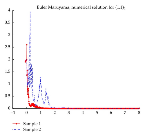
We can see the impact of the Markov chain r(t). The distribution (π = (π₁, π₂, …, π_n)) of r(t) plays a very important role, which, combined with $$, determine that system (1.1) is almost surely exponentially stable. If r(t) spends enough time in the “good” states (the state where ϕ(i) − (q²(i)/2) < 0 for some i), even if there exist some “bad” states (the states where ϕ(i) − (q²(i)/2) > 0 for some i), the system (1.1) will still be almost surely exponentially stable.