Bayesian Networks are graphic probabilistic models through which we can acquire, capitalize on, and exploit knowledge. they are becoming an important tool for research and applications in artificial intelligence and many other fields in the last decade. This paper presents Bayesian networks and discusses the inference problem in such models. It proposes a statement of the problem and the proposed method to compute probability distributions. It also uses D-separation for simplifying the computation of probabilities in Bayesian networks. Given a Bayesian network over a family I of random variables, this paper presents a result on the computation of the probability distribution of a subset S of I using separately a computation algorithm and D-separation properties. It also shows the uniqueness of the obtained result.

1. Introduction

Bayesian networks are graphical models for probabilistic relationships among a set of variables. They have been used in many fields due to their simplicity and soundness. They are used to model, represent, and explain a domain, and they allow us to update our beliefs about some variables when some other variables are observed, which is known as inference in Bayesian networks.

Given a Bayesian network [1] relative to the set X_I = (X_i) _i∈I of random variables, we are interested in computing the joint probability distribution of a nonempty subset S (called target) of I.

The computation of the probability distribution of X_S requires marginalizing out a set of variables of from the joint distribution P_I corresponding to the Bayesian network.

In large Bayesian networks, the computation of probability distributions and conditional probability distributions may require summations relative to very large subsets of I. Consequently there is a need to order and segment, if possible, these computations into several computations that are less intensive and more accessible to a parallel treatment. These segmentations are related to the graphic properties of the Bayesian networks.

This paper describes the computation of P_S using a specific order described by a proposed algorithm, and the segmentations of P_S.

We consider discrete random variables, but the results presented here can be generalized to continuous random variables with the density of X_i relative to a finite measure μ_i (the summations will be replaced by integrations relative to those measures μ_i).

The paper is organized as follows. Section 2 introduces Bayesian networks and Level two Bayesian networks. We, then, present in Section 3 the inference problem in Bayesian networks and the proposed computation algorithm. Section 4 outlines D-Separation in Bayesian networks and describes graphical partitions that will allow the segmentations of the computations of probability distributions. Section 5 proves the uniqueness of the results obtained in Sections 3 and 4.

2. Bayesian Networks and level two Bayesian networks

2.1. Bayesian Networks

A Bayesian network (BN) is a family of random variables (X_i) _i∈I such that:

(i)
the set I is finite and endowed with a structure of a directed acyclic graph (DAG), G, where, for each i:
- (a)
  p(i) is the set of parents of i (p(i) = {j; (j, i) ∈ G})
- (b)
  e(i) is the set of children of i (e(i) = {j; (i, j) ∈ G})
- (c)
  d(i) is the set of descendants of i (d(i) = {k; ∃(ℓ₀, …, ℓ_n) ℓ₀ = i, ℓ_n = k, ∀ s ∈ {1, …, n} (ℓ_s−1, ℓ_s) ∈ G});
(ii)
for each i, X_i is independent of (X_j) _{j∈I−[p(i)∪d(i)]} conditional on X_p(i) (for more details see, e.g., [1–5]).

We know that this is equivalent to the equality

(2.1)

where P_I is the joint probability distribution of X_I = (X_i) _i∈I and P_i/p(i) is the probability distribution of X_i conditional on X_p(i) = (X_j) _j∈p(i).

The joint probability distribution corresponding to the BN in Figure 1 can be written as

(2.2)

Details are in the caption following the image — **Figure 1**
Open in figure viewer PowerPoint

An example of a Bayesian network.

2.2. level two Bayesian networks

We consider the probability distribution P_I of a family (X_i) _i∈I of random variables in a finite space Ω_I = ∏_i∈IΩ_i. Let ℐ be a partition of I and let us consider a DAG 𝒢 on ℐ.

We say that there is a link from J^′ to J^′′ (where J^′ and J^′′ are atoms of the partition ℐ) if (J^′, J^′′) ∈ 𝒢. If J ∈ ℐ, we denote by p(J) the set of parents of J, that is, the set of J^′ such that (J^′, J) ∈ 𝒢.

The probability P_I is defined by the Level Two Bayesian network (BN2), on I, (ℐ, 𝒢, (P_J/p(J)) _J∈ℐ), if for each J ∈ ℐ, we have the conditional probability P_J/p(J), or the probability of X_J conditioned by X_p(J) (which, if p(J) = ∅, is the marginal probability P_J), so that

(2.3)

The probability distribution P_I associated to the BN of level 2 in Figure 2 can be written as

(2.4)

2.3. Close Descendants

We define the set of close descendants of a node J (denoted cd(J)) as the set of vertices containing the children of J and the vertices located on a path between J and one of its children.

In the example below (Figure 2), we have

(2.5)

2.4. Initial Subset

For each subset S, we denote by S⁺ the initial subset defined by S, that is, the set consisting of S itself and the S^′ such that there is a path in 𝒢 from S^′ to S.

We can identify this subset with the union of all S^′ such that S^′ is an ancestor of S

For each S, the Initial subset S⁺ is a BN, in other words the restriction of a BN to an initial subset is a BN

(2.6)

In the example above (Figure 2), we have

(2.7)

3. Inference in Bayesian Networks

Consider the BN in Figure 1.

Suppose we are interested in computing the distribution of S = I − {3}, in other words all variables are in the target S except X₃.

By marginalizing out the variables X₃ from the joint probability distribution P_I, the target distribution P_S can be written as

(3.1)

α is a function that depends on X₁, X₂, X₄, X₅, and X₇ but has nothing to do with P_1,2,4,5,7 joint probability distribution of X₁, X₂, X₄, X₅, X₇.

By doing this we loose the structure of the BN.

If we do the marginalization as follow we obtain (according to Bayes′ theorem):

(3.2)

In other words α(x₁, x₂, x₄, x₅, x₇)P_7/5,6(x₇/x₅, x₆) = P_{5,7,8/1,2,4,6}(x₅, x₇, x₈/x₁, x₂, x₄, x₆).

Which provides S with a structure of a level two Bayesian network shown in Figure 3.

The variables used in the marginalization above, to keep a structure of a BN2, is the the set of close descendants defined above.

More general, if we have to sum out more than one variable there is a need to order the variables first. The aim of the inference will be to find the marginalization, or elimination, ordering for the arbitrary set of variables not in the target. This aim is shared by other node elimination algorithms like “variables elimination” [6], “bucket elimination” [7].

The main idea of all these algorithms is to find the best way to sum over a set of variables from a list of factors one by one. An ordering of these variables is required as an input. The computation depends on the ordering elimination; different elimination ordering produce different factors.

The algorithm we proposed to solve this problem is called the “Successive Restrictions Algorithm” (SRA) [8]. SRA is a goal-oriented algorithm that tries to find an efficient marginalization (elimination) ordering for an arbitrary joint distribution.

The general idea of the algorithm of successive restrictions is to manage the succession of summations on all random variables out of the target S in order to keep on it a structure less constraining than the Bayesian network, but which allows saving in memory; that is the structure of Bayesian Network of Level Two. This was possible using the notion of close descendants.

The principle of the algorithm was presented in details in [8].

4. D-Separation and Computations in a Bayesian Network

We have introduced an algorithm which makes possible the computation of the probability distribution of a subset of random variables (X_s) _s∈S of the initial graph. It is also possible to use the SRA to compute any probability distribution of a set of variables X_A conditionally to another subset X_B (P_A∣B).

This algorithm tries to achieve the target distribution by finding a marginalization ordering that takes into account the computational constraints of the application. It may happen that, in certain simple cases, the SRA would be less powerful than the traditional methods [6, 9–13], but it has the advantages of adapting to any subset of nodes of the initial graph, and also to present in each stage interpretable result in terms of conditional probabilities, and thus technically usable.

In addition to the SRA we propose, especially for large Bayesian networks, to segment the computations into several less heavier computations that could be carried independently. These segmentations are possible using the D-separation.

4.1. D-Separations and Classical Results

Consider a DAG (I, G). A chain is a sequence (x₀, …, x_n) of elements of I such that for all i ≥ 1, (x_i−1, x_i) ∈ G or (x_i, x_i−1) ∈ G.

x₁, …, x_n−1 are called intermediate nodes on this chain.

On an intermediate node x_i a chain can have three connexions as illustrated in Figure 4.

Let (I, G) be a DAG, S⊆I, a and b be distinct nodes in

. A chain between a and b is d-separated by S if there is an intermediate node x satisfying one of the two properties:

(i)
x ∈ S and the connection is, on x, serial or diverging,
(ii)
x ∉ S⁺ and the connection is converging on x.

In other words, A chain is not d-separated by S if it is in a converging connection at each intermediate node of S, and in a serial or a diverging connection at each intermediate node that has no descendants in S.

Classic Result 1 If A and B are d-separated by S. then the variables X_A and X_B are independent conditional on X_S.

4.2. Notions

Given a subset C of I.

Markov Blanket. F(C) of a subset C is made of the parents of C, the children of C and the variables sharing a child with C.
Markov Boundary of C. M(C) = C ∪ F(C)
Close Descent of C. T(C) is the set of all close descendants of the elements in C other that those in C itself.
Exterior Roots of C. R(C) is the set of the parents of the elements of C ∪ T(C) other that those in C ∪ T(C) itself.

As we can see on the following example:

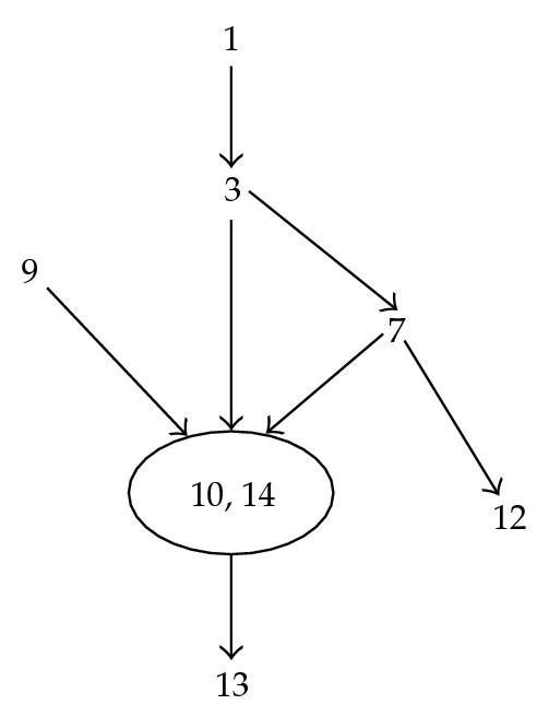
F(C) = {1,10,14,12,9}, M(C) = {3,7, 1,10,14,12,9}, T(3,7) = {10,14,12}, R(3,7) = {1,9}.

Classic Result 2 X_C is d-separated from the rest of the variables conditional on the Markov blanket of C. The proof of these two results and other results related to D-separation can be found in [11].

4.3. Moral and Hypermoral Graphs

Another classic graphic property used with some inference algorithms that we can find in the literature is the notion of the Moral graph.

Moral Graph Given a DAG (I, G)

its associated moral graph is the undirected graph (I, G_m), where G_m is the set

(i)
of pairs {i, j} such that (i, j) ∈ G or (j, i) ∈ G,
(ii)
of pairs {i, j} such that i and j have a child in common.

In a similar way, we define what we call the hypermoral graph defined as follow:

Hypermoral Graph Given a DAG (I, G)

its associated hypermoral graph is the undirected graph (I, G_hm), where G_hm is the set:

(i)
of pairs {i, j} such that (i, j) ∈ G or (j, i) ∈ G,
(ii)
of pairs {i, j} such that i and j have a close descendant in common.

In Figure 5, there is a link between 4 and 7 in the hypermoral graph because they share 9 as a close descendant.

4.4. Moral and Hypermoral Partitions

The moral graph helps defining the moral partition as follow.

(i) We call a S-moral partition the partition of S⁺ − S, denoted , defined by the equivalence relation , where means “ there exists a chain from x to y, in S⁺ − S, not blocked by S.”

In an equivalent way “there exists a chain, in the moral graph G_m, connecting x to y without an intermediate node in S.”

In a similar way we define the hypermoral partition.

(ii) We call an S-hypermoral the partition of S⁺ − S, denoted , defined by the equivalence relation , where means “there exists a chain, in the hypermoral graph G_hm, connecting x to y without an intermediate node in S”. As Illustrated in Figure 6.

4.5. Results

The following results show the possibility of segmenting the computation of the probability distribution P_S.

Theorem 4.1. Let (I, G, P_I) be a BN, and let S be a subset of I. Let be the S-hypermoral partition of S⁺ − S and let K be the set of elements of S which are not close descendants of any element of S⁺ − S, that is, K = {k ∈ S, ∀ y ∈ S⁺ − S, k ∉ cd(y)}. Then,

(4.1)

where

(4.2)

The proof of the theorem can be found in [14].

Theorem 4.2. The set Q_s of singletons {k}, where k ∈ K (if K ≠ ∅), and of subsets T(C)∩S⁺, where , constitutes a partition of S. As Illustrated in Figure 7.

5. Unique Partition

We have seen in the last two sections that the application of the SRA for the computation of P_S provides a structure of BN2, and that the use of D-Separations properties allows the segmentation of the computation of P_S and provides also a structure of a level two Bayesian network on S. In fact the two obtained structures are same, this results is giving by the following theorem.

Theorem 5.1. The following two sets.

(1)
The subsets T(C)∩S⁺, where .
(2)
The set Q_s of singletons {k}, where k ∈ K (if K ≠ ∅)

constitute a unique partition defining a BN2 on S.

Interpretation This theorem indicates that the level two Bayesian network, characterizing the probability distribution P_S, obtained by application of the SRA, is unique independently of the choices done while running the algorithm. This unique partition is constituted of sets of the two types 1 and 2 mentioned above.

Proof. Let us show that the partition of the target S consists of the subsets of types 1 and 2 as mentioned above in the theorem, in other words consists of T(C)∩S⁺ where , and {k} for all k ∈ K.

As S⁺ is a BN-containing S, without a loss of generality, we can limit ourselves to the case where S⁺ = I.

The application of the SRA for the computation of P_S requires marginalizing out the set of variables of following a specific order. Let try to show that the obtained partition by application of the SRA is same mentioned above.

Let us proof this result by induction on the cardinality of .

Let us assume that Card. In this case has only one element, .

On one side, marginalizing out the variable (á) i, by application of the SRA, creates a new node E_i that contains the close descendants of i (i.e., E_i = cd(i)).

The BN2 resulting from this marginalization is formed of the new node E_i along with all other remaining nodes, in other words all the {k} such that k ∈ I − (i₁ ∪ cd(i₁)) = S − E_i, which is shown in Figure 8.

On the other side, since Card, is constituted of a unique equivalent class, C = {i}, so, by definition, the partition of S is constituted of

(1)
T(C)∩S⁺ = cd(i)∩I = cd(i),
(2)
all other nodes, in other words the nodes k ∈ K such that
(5.1)

This shows the result in this first case.

Let us suppose now that Card, and (i₁, …, i_n) as an hierarchical order on .

We are going to sum out following the inverse order of the given hierarchical order.

Let us assume that the result is right till step ℓ (in other words marginalizing out i_n−ℓ+1) and let′s proof the result for step ℓ + 1 (in other words marginalizing out i_n−ℓ).

What justify the proof by induction is that once the marginalizing out i_n, …, i_n−ℓ+1 these last elements will not interfere in the next steps of marginalizing out i_n−ℓ, …, i₁.

The result is right till step ℓ means that we dispose on A = S ∪ {i₁, …, i_n−ℓ}, of a partition that contains the subsets {T(C)∩S⁺} for , and the nodes {k} such that , (i.e., ), where is the S-hypermoral partition associated to A.

Showing the result for ℓ + 1 means to find a partition of S ∪ {i₁, …, i_n−ℓ−1} constituted of subsets of type 1 et 2 mentioned above.

On one hand, let′s first try to find the partition obtained by application of the SRA. We know that, the marginalization of i_n−ℓ creates a new node, , which contains the close descendants of i_n−ℓ in the BN2 on A (), shown by Figure 9.

So if we write J = {k₁, …, k_r}, the set of K such that for all j ∈ {1, …, r}, and L = {C₁, …, C_m}, the set of such that for all s ∈ {1, …, m}, T(C_s)∩cd(i_n−ℓ) ≠ ∅.

In this case, the partition of B = A − {i_n−ℓ} = S ∪ {i₁, …, i_n−ℓ−1} is constituted of the new node , and all the other nodes that are left isolated, in other words all the nodes k ∈ (K − J) and all the {T(C)∩A⁺} where .

If we write so the partition of B by application of the SRA is composed of the following two types of sets:

(1)
,
(2)
all other isolated nodes, that is, the nodes of K^′.

On the other hand, let′s now try to determine the partition of B = A − {i_n−ℓ} using the D-Separation properties.

We have on A a partition composed of nodes {T(C)∩A⁺} where , and all nodes {k} such that .

Since B = A − {i_n−ℓ}, and no descendant of i_n−ℓ is in i₁, …, i_n−ℓ−1, (by definition of the hierarchical order), so only one equivalent subset is associated, , it results by definition, the partition of B = S ∪ {i₁, …, i_n−ℓ−1} is composed of the following types of subsets:

(1)
,
(2)
all other isolated nodes R such that
(5.2)

So we have .

This shows that this partition is same partition obtained by application of the SRA.

References

1 Jensen F. V., An Introduction to Bayesian Networks, 1999, UCL Press.
Google Scholar
2 Jensen F. V., Lauritzen S. L., and Olesen K. G., Bayesian updating in causal probabilistic networks by local computations, Computational Statistics Quarterly. (1990) 5, no. 4, 269–282, 1073446, ZBL0715.68076.
Google Scholar
3 Spirtes P., Glymour C., and Scheines R., Causation, Prediction, and Search, 1993, 81, Springer, New York, NY, USA, Lecture Notes in Statistics, 1227558.
10.1007/978-1-4612-2748-9
Web of Science® Google Scholar
4 Dan G. and Pearl J., Axioms and algorithms for inferences involving conditional independence, 1989, no. CSD 890031, R-119-I, Cognitive Systems Laboratory, University of California, Los Angeles, Calif, USA.
Google Scholar
5 Heckerman D., M. Jordan, A tutorial on learning with Bayesian networks, Learning in Graphical Models, 1999, MIT Press, Cambridge, Mass, USA.
Google Scholar
6 Zhang N. L. and Poole D., A simple approach to bayesian network computations, Proc. of the Tenth Canadian Conference on Artificial Intelligence, 1994, 171–178.
Google Scholar
7 Dechter R., Bucket elimination: a unifying framework for probabilistic inference, Uncertainty in Artificial Intelligence, 1996, Morgan Kaufmann, San Francisco, Calif, USA, 211–219, 1617213.
Google Scholar
8 Smail L. and Raoult J. P., A. F. Famili et al., Successive restrictions algorithm in Bayesian networks, 3646, Proceedings of the International Symposium on Intelligent Data Analysis (IDA ′05), 2005, Berlin, Germany, Springer, 409–418, Lecture Notes in Computer Science.
Google Scholar
9 Cowell R. G., Dawid A. P., Lauritzen S. L., and Spiegelhalter D. J., Probabilistic Networks and Expert Systems, 1999, Springer, New York, NY, USA, Statistics for Engineering and Information Science, 1697175.
Google Scholar
10 Neapolitan R. E., Probabilistic Reasoning in Expert Systems, 1990, John Wiley & Sons, New York, NY, USA, A Wiley-Interscience Publication, 1044998.
Google Scholar
11 Pearl J., Probabilistic Reasoning in Intelligent Systems: Networks of Plausible Inference, 1988, Morgan Kaufmann, San Francisco, Calif, USA, The Morgan Kaufmann Series in Representation and Reasoning, 965765.
Google Scholar
12 Hájek P., Havránek T., and Jiroušek R., Uncertain Information Processing in Expert Systems, 1992, CRC Press, Boca Raton, Fla, USA, 1253068.
Google Scholar
13 Shafer G., Probabilistic Expert Systems, 1996, 67, SIAM, Philadelphia, Pa, USA, CBMS-NSF Regional Conference Series in Applied Mathematics, 1400892.
10.1137/1.9781611970043
Google Scholar
14 Smail L., D-separation and level two Bayesian networks, Artificial Intelligence Review. (2009) 31, no. 1–4.
10.1007/s10462-009-9128-3
Web of Science® Google Scholar

Citing Literature

All articles

Uniqueness of the Level Two Bayesian Network Representing a Probability Distribution

Abstract

1. Introduction