We present an explicit formula which unifies the mask of (2n − 1)-point ternary interpolating as well as approximating subdivision schemes. We observe that the odd point ternary interpolating and approximating schemes introduced by Lian (2009), Siddiqi and Rehan (2010, 2009) and Hassan and Dodgson (2003) are special cases of our proposed masks/schemes. Moreover, schemes introduced by Zheng et al. (2009) can easily be generated by our proposed masks. It is also proved from comparison that (2n − 1)-point schemes are better than 2n-scheme in the sense of computational cost, support and error bounds.

1. Introduction

Subdivision is an algorithmic technique to generate smooth curves and surfaces as a sequence of successively refined control polygons. The schemes involving convex combination of more or less than six points at coarse refinement level to insert a new point at next refinement level is introduced by [1–8]. They introduced odd and even points ternary schemes. Zheng et al. [9] constructed (2n − 1)-point ternary interpolatory subdivision schemes by using variation of constants. They also introduced ternary even symmetric 2n-point subdivision schemes [10]. Mustafa and Khan [11] presented a new 4-point C³ quaternary approximating subdivision scheme. Lian [12] generalized 3-point and 5-point interpolatory schemes into an a-ary subdivision scheme for curve design. Later on, he further generalized his work into 2m-point and (2m + 1)-point interpolating a-ary schemes for curve design [13]. Mustafa and Najma [14] generalized and unified even-point n-ary interpolating and approximating subdivision schemes for any n⩾2. In this paper, we introduce an explicit formula which generalizes and unifies existing odd-point ternary interpolating and approximating subdivision schemes. A general formula which unifies odd-point and even-point n-ary interpolating and approximating schemes is still under investigation.

2. Preliminaries

Let ℤ be the set of integers and α = {a_j, b_j, j = −(n − 1), …, (n − 1), n ≥ 2} be the set of constants. A general form of (2n − 1)-point ternary subdivision scheme S which relates a set of control points

to refined set of control points

is defined by

(2.1)

Which is formally denoted by f^k+1 = Sf^k. The set α of constants is called mask of the scheme S. A necessary condition for the uniform convergence of the subdivision scheme (2.1) given by [3] is

(2.2)

The Laurent polynomial

(2.3)

corresponding to the mask of convergent subdivision scheme (2.1) satisfies

(2.4)

For the given n, we define Lagrange fundamental polynomials of degree 2n − 2, at the points −(n − 1), −(n − 2), …, (n − 1), by

(2.5)

and Lagrange fundamental polynomials of degree 2n − 3 at the points −(n − 2), −(n − 3), …, (n − 1), by

(2.6)

3. (2n − 1)-Point Ternary Approximating and Interpolating Schemes

Here, first we present some preliminary identities then we will offer masks of (2n − 1)-point ternary approximating and interpolating schemes.

Lemma 3.1. If is Lagrange fundamental polynomial of degree 2n − 2 corresponding to nodes defined by (2.5), then

(3.1)

where j = −(n − 1), …, (n − 1).

Proof. Consider

(3.2)

This implies

(3.3)

This further implies

(3.4)

This can be written as

(3.5)

where j = −(n − 1)⋯(n − 1). It is easy to verify that

(3.6)

Now by substituting (3.5), (3.6), and x = −1/3 in (2.5), we get (3.1).

This completes the proof.

Similarly, we can prove the following lemma.

Lemma 3.2. If is Lagrange fundamental polynomial of degree 2n − 3 corresponding to nodes defined by (2.6) then

(3.7)

where j = −(n − 2), …, (n − 1).

Lemma 3.3. If and are Lagrange polynomials defined by (2.5) and (3.1), then

(3.8)

where j = −(n − 2), …, (n − 1).

Proof. By (3.1), for j = −(n − 1), we get

(3.9)

Using (3.1), (3.7), and (3.9), we get (3.8). This completes the proof.

Remark 3.4. In the setting of primal parametrization, each ternary refinement of coarse polygon of scheme (2.1) replaces the old data by new data and , one to the left, the other to the right, and both at one-third the distance to the neighbours and . In other words, ternary refinement (2.1) defines a scheme whereby replaces the value at the mesh point and and are inserted at the new mesh point and , respectively.

Therefore, we can select the value of x either 1/3 or 2/3 to prove the Lemmas 3.1–3.3. In this paper, x = 1/3 has been selected. One can select x = 2/3 to proof the above lemmas. The results of the above lemmas at x = ± 1/3 are same but the final mask of the scheme obtained in reverse order. Negative values give a proper order of the mask, that have why negative values have been selected to prove the above lemmas.

Now here we present the masks of (2n − 1)-point ternary approximating and interpolating schemes.

Theorem 3.5. An explicit formula for the mask of (2n − 1)-point ternary scheme (2.1) is defined by

(3.10)

where u is free parameter while β_j, χ_j, and β are defined by (3.7), (3.8), and (3.9) respectively.

3.1. 3-, 5-, 7-Point Ternary Approximating Schemes

Here, we present three special cases of approximating schemes generated by (3.10) with free parameter.

(i)
If n = 2 then by (2.1) and (3.10), we get the following 3-point ternary approximating scheme:

(3.11)

(ii)
If n = 3 then by (2.1) and (3.10), we get the following 5-point ternary approximating scheme:

(3.12)

(iii)
If n = 4 then by (3.10), we get the following mask of 7-point ternary approximating scheme:
(3.13)
where
(3.14)

3.2. 3-, 5-Point Ternary Interpolating Schemes

Here, we present two special cases of approximating schemes generated by (3.10) with free parameters.

(i)
By setting n = 2 and u = β, we get the following 3-point ternary interpolating scheme:

(3.15)

(ii)
If n = 3 and u = β, then by (2.1) and (3.10), we get the following 5-point ternary interpolating scheme:

(3.16)

3.3. Comparison with Existing Ternary Schemes

In this section, we will show that the popular existing odd-point ternary schemes are special cases of our proposed family of scheme. Here we will also compare the error bounds between limit curve and control polygon after k-fold subdivision of odd-point and even-point schemes.

3.3.1. Special Cases

Here we see that the most of the existing odd-point ternary subdivision schemes are either special cases or can be obtain by setting free parameter in our proposed masks.

(i)
By letting u = β in (3.10), Zheng et al. (2n − 1)-point interpolating scheme [9] becomes special case of our scheme.
(ii)
By substituting u = 2/9, and u = −7/243 in (3.15) and (3.16), we get 3-point and 5-point ternary interpolating schemes of Lian [12] respectively.
(iii)
By substituting u = 35/6561 in (3.13), we get 7-point ternary interpolating scheme of Lian [13]. Similarly, from (3.10), we can generate (2m + 1)-point ternary interpolating schemes of [13].
(iv)
For n = 2, and parameter u = μ + 25/72 in our proposed mask (3.13), 3-point ternary approximating scheme given in [7] becomes special case of our scheme.
(v)
For n = 2, and u = 10/27 in (3.11), we get 3-point approximating scheme of Hassan and Dodgson [4].
(vi)
For n = 2, b = u = 2/9 and a = u − 1/3 in (3.11), we get 3-point interpolating scheme of Hassan and Dodgson [4].

3.3.2. Error Bounds

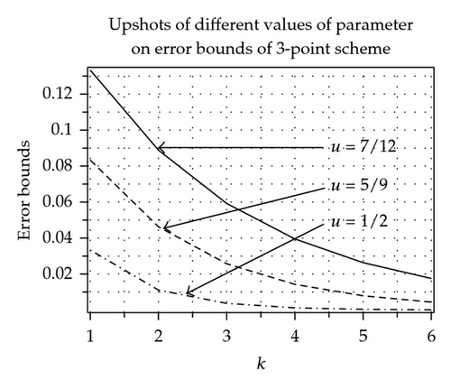
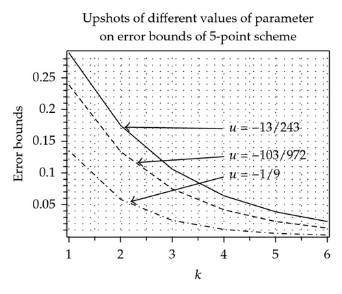
In Tables 1 and 2 by using [15], with χ = 0.1, we have computed error bounds between limit curve and control polygon after k-fold subdivision of odd-point and even-point ternary approximating and interpolating schemes. It is clear from Tables 1 and 2 that error bounds of 3-point ternary schemes (3.11) and (3.15) at each subdivision level k are less than the error bounds of 4-point ternary schemes [3, 10] at each level. Similarly error bounds of 5-point scheme (3.12) and (3.16) are less than the error bounds of 6-point schemes [10, 16]. Similar results can be obtained by comparing other odd-point and even-point schemes. Graphical representation of error bounds is shown in Figure 1.

Table 1. Error bounds of odd-point and even-point ternary interpolating schemes.

k	1	2	3	4	5	6
3-point	0.033333	0.011111	0.003704	0.001235	0.000412	0.000137
4-point [10]	0.082821	0.034969	0.104765	0.006234	0.002632	0.001111
5-point	0.136205	0.058854	0.025431	0.010989	0.004748	0.002052
6-point [10]	0.199159	0.094908	0.045228	0.021553	0.010271	0.004895

Table 2. Error bounds of odd-point and even-point ternary approximating schemes.

k	1	2	3	4	5	6
3-point	0.133333	0.088889	0.059259	0.039506	0.26337	0.017558
4-point [3]	0.203672	0.129495	0.082333	0.052348	0.33283	0.021161
5-point	0.289236	0.174970	0.105846	0.064030	0.38734	0.023432
6-point [16]	0.429283	0.285291	0.189598	0.126002	0.83738	0.055650

Details are in the caption following the image — **Figure 1 (a)**
Open in figure viewer PowerPoint

Comparison: error bounds between kth level control polygon and limit curves of different subdivision schemes.

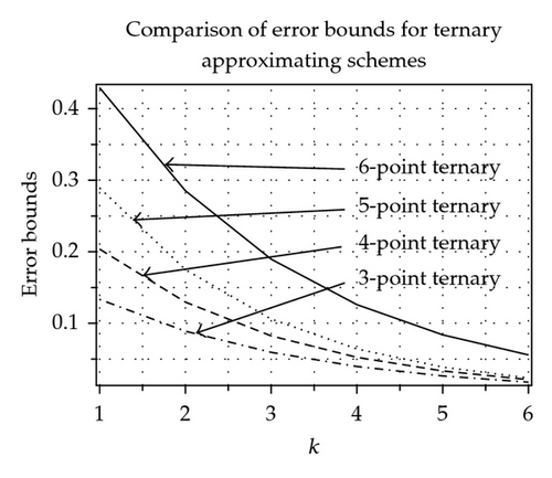
Moreover, support and computational cost of (2n − 1)-point schemes are less than 2n-point schemes. Therefore, we conclude that (2n − 1)-point schemes are better than 2n-point schemes in the sense of support, computational cost, and error bounds.

3.4. Effects of Parameters in Proposed Schemes

We will discuss three major effects/upshots of parameter in schemes (3.11)–(3.16). Effect of parameters in other schemes can be discuss analogously.

3.4.1. Continuity

The effect/upshots of parameter u in schemes (3.11)–(3.16) on order of continuity is shown in Tables 3 and 4. One can easily find the order of continuity over parametric intervals by using approach of [4].

Table 3. The order of continuity of proposed 3-, 5-, and 7-point ternary approximating schemes for certain ranges of parameter.

Scheme	Parameter	Continuity
	1/6 < u < 2/3	C⁰
3-point	2/9 < u < 5/9	C¹
	1/3 < u < 4/9	C²

5-point	−11/81 < u < −7/648	C⁰
	−103/972 < u < −11/486	C¹
	−2/27 < u < −49/972	C²
	−1/18 < u < −38/729	C³

7-point	7/23328 < u < 23/729	C⁰
	157/52488 < u < 2501/104976	C¹
	1043/104976 < u < 67/4374	C²
	53/8748 < u < 187/17496	C³

Table 4. The order of continuity of proposed 3- and 5-point ternary interpolating schemes for certain ranges of parameter.

Scheme	Parameter	Continuity
3-point	1/6 < u < 2/3	C⁰
3-point	2/9 < u < 1/3	C¹

	−11/81 < u < −7/648	C⁰
5-point	−17/324 < u < −2/81	C¹
	−5/108 < u < −7/162	C²

3.4.2. Shapes of Limit Curves

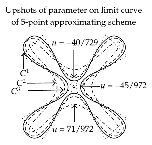
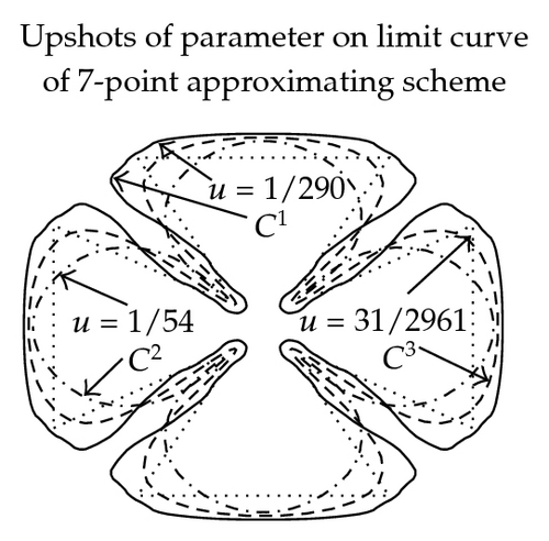
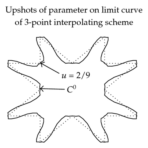
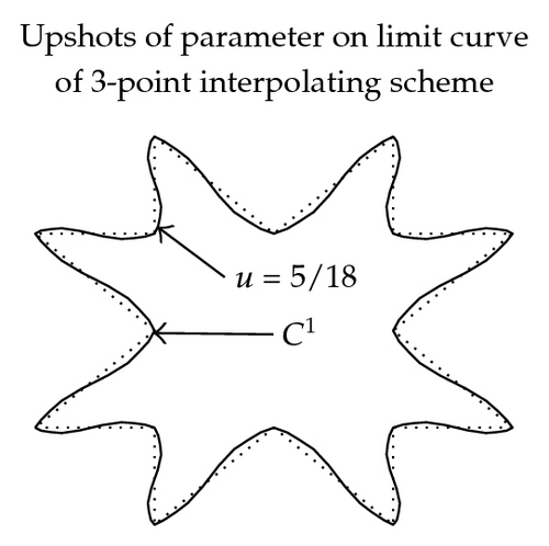
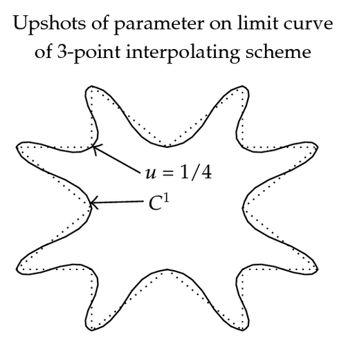
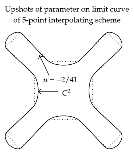
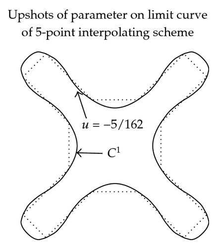
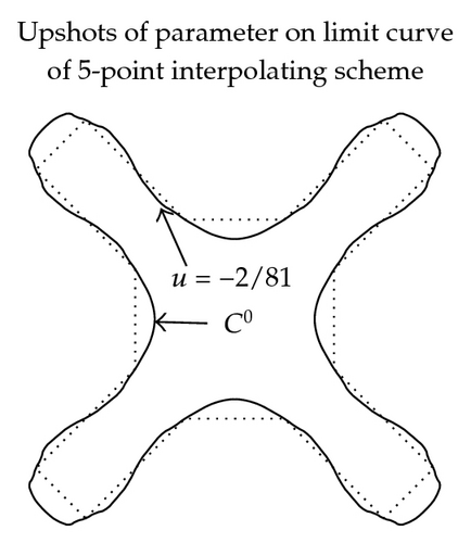
In Figure 2, the effect of parameter in (3.11)–(3.16) on graph and continuity of limit curve is shown. These figures are exposed to show the role of free parameter when 3- and 5-point approximating and interpolating schemes (3.11)–(3.16) applied on discrete data points. From these figures, we see that the behavior of the limiting curve acts as tightness/looseness when the values of free parameter vary.

3.4.3. Error Bounds

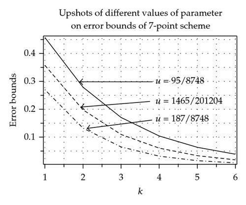
The effects of parameter on error bounds at each subdivision level between kth level control polygon and limit curves are shown in Figure 3, Tables 5 and 6. From these tables and figures, we conclude that in case of 3-point approximating scheme continuity is maximum over 1/3 < u < 4/9 and error bound is minimum over 1/3 ≤ u ≤ 1/2. On each side of interval 1/3 < u < 4/9 continuity decreases while error bounds increases on each side of interval 1/3 ≤ u ≤ 1/2. In case of 5-, 7-point approximating scheme continuity is maximum over −1/18 < u < −38/729 and 53/8748 < u < 187/17496, while error bound is minimum at u = −13/243 and u = 95/8748, respectively.

Table 5. Error bounds for 3-, 5- and 7-point ternary approximating subdivision schemes.

Scheme	Parameter	k = 1	k = 2	k = 3	k = 4	k = 5	k = 6
	u = 1/2	0.033333	0.011111	0.003703	0.001234	0.000411	0.000137
3-point	u = 5/9	0.083333	0.046296	0.025720	0.014289	0.007938	0.004410
	u = 7/12	0.133333	0.088889	0.059259	0.039506	0.026337	0.017558

	u = −13/243	0.134953	0.058313	0.025197	0.010888	0.004704	0.002033
5-point	u = −103/972	0.238775	0.133636	0.074792	0.041859	0.023427	0.013112
	u = −1/9	0.289236	0.174970	0.105846	0.064030	0.038734	0.023432

	u = 95/8748	0.270022	0.132233	0.064756	0.031712	0.015530	0.007605
7-point	u = 1465/201204	0.357567	0.197809	0.109430	0.060538	0.033490	0.018527
	u = 187/8748	0.457353	0.279180	0.170418	0.104028	0.063501	0.038763

Table 6. Error bounds for 3- and 5-point ternary interpolating subdivision schemes.

Scheme	Parameter	k = 1	k = 2	k = 3	k = 4	k = 5	k = 6
	u = 1/3	0.033333	0.011111	0.003703	0.001234	0.000411	0.000137
3-point	u = 7/18	0.053333	0.023704	0.010535	0.004682	0.002081	0.000925
	u = 5/18	0.097222	0.054012	0.030007	0.016670	0.009261	0.005145

	u = −2/41	0.136205	0.058854	0.025431	0.010989	0.004748	0.002052
5-point	u = −7/162	0.169665	0.081691	0.039332	0.018938	0.009118	0.004390
	u = −1/27	0.257698	0.149528	0.086763	0.050344	0.029212	0.016950

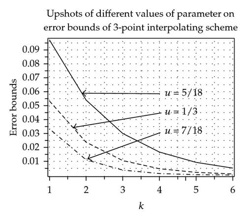
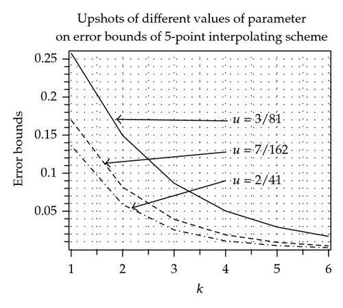
While in case of 3- and 5-point interpolating scheme continuity is maximum over 2/9 < u < 1/3 and −5/108 < u < −7/162, while error bound is minimum at u = 1/3 and u = −2/41, respectively.

3.5. Conclusion

In this paper, we offered an explicit general formula for the generation of mask of (2n − 1)-point ternary interpolating as well as approximating schemes. We have concluded from figures and tables that the (2n − 1)-point schemes are better than 2n-point schemes for n ≥ 2 in the sense of computational cost, support and error bounds. Moreover, odd-point ternary schemes of Hassan and Dodgson [4], Lian [12, 13], Zheng et al. [9], and Siddiqi and Rehan [7, 8] are special cases of our proposed masks.

Acknowledgment

This work is supported by the Indigenous Ph.D. Scholarship Scheme of Higher Education Commission (HEC), Pakistan.

References

1 Beccari C., Casciola G., and Romani L., An interpolating 4-point C² ternary non-stationary subdivision scheme with tension control, Computer Aided Geometric Design. (2007) 24, no. 4, 210–219, https://doi.org/10.1016/j.cagd.2007.02.001, 2320435, ZBL1171.65326.
10.1016/j.cagd.2007.02.001
Web of Science® Google Scholar
2 Deslauriers G. and Dubuc S., Symmetric iterative interpolation processes, Constructive Approximation. (1989) 5, no. 1, 49–68, Fractal approximatiohttps://doi.org/10.1007/BF01889598, 982724, ZBL0659.65004.
10.1007/BF01889598
Web of Science® Google Scholar
3 Hassan M. F., Ivrissimitzis I. P., Dodgson N. A., and Sabin M. A., An interpolating 4-point C² ternary stationary subdivision scheme, Computer Aided Geometric Design. (2002) 19, no. 1, 1–18, https://doi.org/10.1016/S0167-8396(01)00084-X, 1879678.
10.1016/S0167-8396(01)00084-X
Web of Science® Google Scholar
4 Hassan M. F. and Dodgson N. A., A. Cohen, J. L. Marrien, and L. L. Schumaker, Ternary and three-point univariate subdivision schemes, Curve and Surface Fitting: Saint-Malo, 2002, 2003, Nashboro Press, Brentwood, Tenn, USA, 199–208, 2042447, ZBL1037.65024.
Google Scholar
5 Khan F. and Mustafa G., Ternary six-point interpolating subdivision scheme, Lobachevskii Journal of Mathematics. (2008) 29, no. 3, 153–163, https://doi.org/10.1134/S1995080208030062, 2434894.
10.1134/S1995080208030062
Google Scholar
6 Ko K. P., Lee B.-G., and Yoon G. J., A ternary 4-point approximating subdivision scheme, Applied Mathematics and Computation. (2007) 190, no. 2, 1563–1573, https://doi.org/10.1016/j.amc.2007.02.032, 2339748, ZBL1144.65012.
10.1016/j.amc.2007.02.032
Web of Science® Google Scholar
7 Siddiqi S. S. and Rehan K., Modified form of binary and ternary 3-point subdivision schemes, Applied Mathematics and Computation. (2010) 216, no. 3, 970–982, https://doi.org/10.1016/j.amc.2010.01.115, 2607005, ZBL1198.65042.
10.1016/j.amc.2010.01.115
Web of Science® Google Scholar
8 Siddiqi S. S. and Rehan K., A stationay ternary C⁴ scheme for curve sketching, European Journal of Scientific Research. (2009) 30, no. 3, 380–388.
Google Scholar
9 Zheng H., Hu M., and Peng G., Constructing (2n − 1)-point ternary interpolatory subdivision schemes by using variation of constants, Proceedings of the International Conference on Computational Intelligence and Software Engineering (CiSE ′09), 2009, Wuhan, China, https://doi.org/10.1109/CISE.2009.5364446.
10.1109/CISE.2009.5364446
Google Scholar
10 Zheng H., Hu M., and Peng G., Ternary even symmetric 2n-point subdivision, Proceedings of the International Conference on Computational Intelligence and Software Engineering (CiSE ′09), 2009, Wuhan, China, https://doi.org/10.1109/CISE.2009.5363033.
10.1109/CISE.2009.5363033
Google Scholar
11 Mustafa G. and Khan F., A new 4-point C³ quaternary approximating subdivision scheme, Abstract and Applied Analysis. (2009) 2009, 14, https://doi.org/10.1155/2009/301967, 301967, 2515998, ZBL1167.65342.
10.1155/2009/301967
Google Scholar
12 Lian J.-A., On α-ary subdivision for curve design. II. 3-point and 5-point interpolatory schemes, Applications and Applied Mathematics. (2008) 3, no. 2, 176–187, 2469964.
Google Scholar
13 Lian J.-A., On α-ary subdivision for curve design. III. 2m-point and (2m + 1)-point interpolatory schemes, Applications and Applied Mathematics. (2009) 4, no. 2, 434–444, 2579550.
Google Scholar
14 Mustafa G. and Najma A. R., The mask of (2b + 4)-point n-ary subdivision scheme, Computing. (2010) 90, no. 1-2, 1–14, https://doi.org/10.1007/s00607-010-0108-x, 2719780.
10.1007/s00607-010-0108-x
Web of Science® Google Scholar
15 Mustafa G. and Deng J., Estimating error bounds for ternary subdivision curves/surfaces, Journal of Computational Mathematics. (2007) 25, no. 4, 473–483, 2337408, ZBL1141.65341.
Web of Science® Google Scholar
16 Mustafa G. and Ashraf P., A new 6-point ternary interpolating subdivision scheme and its differentiability, Journal of Information and Computing Science. (2010) 5, no. 3, 199–210.
Google Scholar

Citing Literature

All articles

(2n − 1)-Point Ternary Approximating and Interpolating Subdivision Schemes

Abstract

1. Introduction

2. Preliminaries

3. (2n − 1)-Point Ternary Approximating and Interpolating Schemes

3.1. 3-, 5-, 7-Point Ternary Approximating Schemes

3.2. 3-, 5-Point Ternary Interpolating Schemes