In the presence of a risk-free asset the investment opportunity set obtained via the Markowitz portfolio optimization procedure is usually characterized in terms of the vector of excess returns on individual risky assets and the variance-covariance matrix. We show that the investment opportunity set can alternatively be characterized in terms of the vector of Sharpe ratios of individual risky assets and the correlation matrix. This implies that the changes in the characteristics of individual risky assets that preserve the Sharpe ratios and the correlation matrix do not change the investment opportunity set. The alternative characterization makes it simple to perform a comparative static analysis that provides an answer to the question of what happens with the investment opportunity set when we change the risk-return characteristics of individual risky assets. We demonstrate the advantages of using the alternative characterization of the investment opportunity set in the investment practice. The Sharpe ratio thinking also motivates reconsidering the CAPM relationship and adjusting Jensen′s alpha in order to properly measure abnormal portfolio performance.

1. Introduction

The mean-variance model of asset choice has been proposed by Markowitz [1] and used extensively in finance principally due to a strong intuitive appeal and the existence of closed-form solutions to the optimal portfolio choice and equilibrium problems. The papers by Merton [2] and Roll [3] are the two seminal papers where the authors provide a rigorous characterization of the investment opportunity set in the absence and in the presence of a risk-free asset.

In the absence of a risk-free asset the investment opportunity set is characterized by the vector of expected returns on risky assets and the variance-covariance matrix. In the presence of a risk-free asset the investment opportunity set is characterized by the vector of excess returns on risky assets and the variance-covariance matrix. To demonstrate the classical characterization of the investment opportunity set one typically employs a two-dimensional standard deviation-expected return space. Next one illustrates the construction of the minimum-variance frontier of risky assets. In the absence of a risk-free asset the efficient part of the minimum-variance frontier of risky assets coincides with the investment opportunity set. In the presence of a risk-free asset one draws a straight line (whose intercept and slope are equal to the risk-free rate of return and the maximum Sharpe ratio, resp.) which is tangent to the efficient frontier of risky assets.

In this paper we show that in the presence of a risk-free asset the investment opportunity set can alternatively be characterized in terms of the vector of the Sharpe ratios of risky assets and the correlation matrix. This implies that the changes in the characteristics of individual risky assets that preserve the Sharpe ratios of risky assets and the correlation matrix do not change the investment opportunity set. In other words, two apparently different sets comprised of the same number of risky assets (different in terms of the values of expected returns and standard deviations), that produce apparently different minimum-variance frontiers of risky assets, will generate exactly the same investment opportunity set if the risky assets in the two sets have the same Sharpe ratios and correlation matrix.

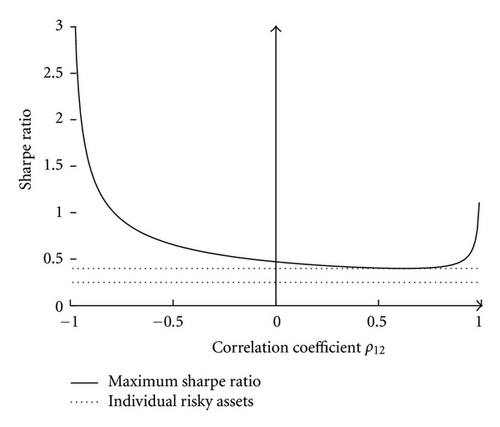
The alternative characterization of the investment opportunity set in the presence of a risk-free asset implies that the two-dimensional standard deviation-expected return space, although instructive in teaching, can be redundant and misleading in practice. A more straightforward depiction of the characteristics of individual risky assets and the investment opportunity set can be done in one-dimensional Sharpe ratio space. For the case of two risky assets the alternative characterization allows to visualize the maximum Sharpe ratio as a function of the correlation coefficient.

In addition, the alternative characterization of the investment opportunity set provides a simple answer to the question of what happens with the investment opportunity set when we change the risk-return characteristics of individual risky assets. In other words, if we change the values of the expected returns and standard deviations of individual risky assets, will it result in an improvement or worsening of the investment opportunity set? Using the classical characterization of the investment opportunity set, the answer is not clear. With the alternative characterization of the investment opportunity set by means of the Sharpe ratios of individual risky assets, the answer is rather trivial. We show that if the weight of a risky asset in the optimal risky portfolio is positive, then an increase in the Sharpe ratio of this asset results in an improvement of the investment opportunity set. Moreover, if the market is in equilibrium, then an increase in the Sharpe ratio of any risky asset results in an increase in the maximum Sharpe ratio.

Finally, the alternative characterization of the investment opportunity set has a clear appeal to the investment practice. In particular, it is well known that the risk-return characteristics of individual risky assets and the correlations among them are changing over time. Existing academic studies usually address only the changing nature of correlations and try to deduce how these changes affect the investment opportunity set. The alternative characterization of the investment opportunity set motivates the idea that one also needs to examine the changing nature of the Sharpe ratios, in addition to that of the correlation structure, in order to have a full picture of the evolution of the investment opportunity set.

The classical CAPM is, in fact, none other than the Markowitz portfolio theory in the presence of a risk-free asset combined with an equilibrium condition. Therefore, the Sharpe ratio thinking motivates reconsidering the CAPM relationship in terms of Sharpe ratios. We show that the classical expected return-beta relationship can alternatively be represented by a Sharpe ratio-rho relationship (rho denotes the correlation coefficient between the returns on a risky asset and the market portfolio). Moreover, the Sharpe ratio thinking motivates adjusting Jensen′s alpha in order to properly measure abnormal portfolio performance. Instead of Jensen′s alpha we propose to use Jensen′s alpha divided by the total risk. In this manner the adjusted Jensen′s alpha becomes a true reward-to-risk performance measure that cannot be manipulated by leverage.

The rest of the paper is organized as follows. In Section 2 we review the classical characterization of the investment opportunity set in the presence of a risk-free asset. In Section 3 we derive the alternative characterization of the investment opportunity set and perform a comparative static analysis. In this section we also present several theoretical examples and one real-world example that illustrate the derived relationships and demonstrate the advantages of the alternative characterization of the investment opportunity set. In Section 4 we reconsider the CAPM relationship and introduce an adjusted Jensen′s alpha. Section 5 summarizes the paper.

2. The Maximum Sharpe Ratio

The purpose of this section is to introduce the notation, the investor′s optimal portfolio choice problem, and to derive the expression for the maximum Sharpe ratio that characterizes the investment opportunity set in the presence of a risk-free asset. We do not provide all details of the derivation because there are no new results in this section. Our exposition in this section is similar to that in Huang and Litzenberger [4, Chapter 3].

We suppose that the investment universe consists of n + 1 assets with returns x_i, i = 1, …, n. Asset 0 is a risk-free asset which provides a return of r. The market is frictionless and the assets can be bought and sold short without any limitations. We suppose that the investor allocates a proportion w_i of his wealth to asset i. That is, the return on the investor′s complete portfolio is given by

(1)

This allows us to write the return on the complete portfolio as

(2)

We denote the expected return on asset x_i by E[x_i] and the variance by

. We also denote Cov(x_i, x_j) = σ_ij = ρ_ijσ_iσ_j, where ρ_ij = ρ_ji is the correlation coefficient between the returns on assets i and j. In matrix notation the vectors of expected returns on the risky assets, the portfolio weights of the risky assets, and the variance-covariance matrix are given by

(3)

Consequently, in matrix notation

(4)

where 1 is a vector of ones. We suppose that the return on any risky asset cannot be expressed as a linear combination of the returns on other assets. Under this assumption, asset returns are linearly independent and the variance-covariance matrix is nonsingular (which also means that it is invertible). The variance-covariance matrix is symmetric because σ_ij = σ_ji. Since the portfolio variance is positive, we conclude that the variance-covariance matrix is positive definite.

We further suppose that the investor exhibits mean-variance preferences. In particular, this investor prefers portfolios that have minimum variance for various levels of expected rate of return. The classical Markowitz portfolio optimization procedure consists in finding a portfolio that has minimum variance for a given level of expected return, μ. That is, w is a solution to the following quadratic program:

(5)

Forming the Lagrangian, we know that w is the solution to the following:

(6)

Since matrix V is positive definite, this insures that the first-order condition is necessary and sufficient for a global minimum. The first-order condition for the optimality of w gives

(7)

Solving with respect to w, we obtain

(8)

The investment opportunity set is defined as all risk-return combinations available to the investor. The computation of the variance of the minimum-variance portfolio gives

(9)

It is easy to observe that in the standard deviation—expected return plane the investment opportunity set represents a straight line:

(10)

where

(11)

denotes the slope of this straight line. Note that since

(12)

can be interpreted as the Sharpe ratio of any portfolio in the investment opportunity set (excluding the case where E[x_p] = r). Observe that the Sharpe ratio of any portfolio in the investment opportunity set has the maximum Sharpe ratio among all feasible portfolios x_p that satisfy the condition

. Therefore, we will refer to

as the maximum Sharpe ratio. Consequently, the investment opportunity set in the presence of a risk-free asset can be characterized by the maximum Sharpe ratio. Finally recall that the investment opportunity set is tangent to the efficient frontier of risky assets. The composition of the tangency portfolio is the same as the composition of any risky portfolio in the investment opportunity set and the weights of the tangency portfolio must sum up to 1. This gives us

(13)

Note that (this will be used later in the paper)

(14)

since for a portfolio in the investment opportunity set μ − r > 0 and

. The combination of (13) and (8) gives us the following expression for the weights of risky assets in the tangency portfolio:

(15)

3. Alternative Characterization of the Maximum Sharpe Ratio

First we introduce the vector of the Sharpe ratios of individual risky assets and the correlation matrix

(16)

Note that since matrix V is invertible and matrix R is essentially a normalized version of matrix V, this means that matrix R is also invertible. Now we are ready to state the main result.

Theorem 1. The maximum Sharpe ratio can be characterized in terms of the vector of Sharpe ratios of individual risky assets and the correlation matrix. In particular,

(17)

Proof. Define the diagonal matrix of standard deviations of the returns on individual risky assets

(18)

Since the entries σ₁, …, σ_n of the diagonal matrix are all nonzero, the diagonal matrix of standard deviations is invertible. The variance-covariance matrix can, thus, be written as (note that symmetry of Σ implies Σ^′ = Σ)

(19)

Since matrixes Σ and R are invertible,

(20)

Consequently, the maximum Sharpe ratio can be rewritten as (now note that, since Σ is symmetric, Σ⁻¹ is also symmetric)

(21)

Let us find the expression for

(22)

where det (Σ) and adj(Σ) are the determinant and the adjoint of Σ, respectively, and Σ_ij is an element of the cofactor matrix of Σ. Since all off-diagonal elements of Σ are zeros, we arrive at

(23)

Note that, whereas det (Σ) is a product of all σ_k (k ∈ [1, …, n]), Σ_ii is a product of all σ_k except σ_i. Consequently,

(24)

Consider the vector Σ⁻¹(e − 1r). It equals

(25)

Finally, (21) for the maximum Sharpe ratio can be rewritten as (17).

Corollary 1. In case the returns on the risky assets in the investment universe are not correlated, that is, ρ_ij = 0 for i ≠ j, then the maximum Sharpe ratio equals

(26)

Proof. In this case R = I_n where I_n is the identity matrix of order n. For the identity matrix . Consequently,

(27)

Now we turn to the presentation of some examples.

Example 1 (n = 1). In this simplest case the investment universe consists of one risky asset and a risk-free asset. The application of (17) gives

(28)

which means that the maximum Sharpe ratio equals the Sharpe ratio of the single risky asset (supposing that S(x₁) > 0).

Example 2 (n = 2 with graphical illustration). In this case the investment universe consists of two risky assets and a risk-free asset. The computation of the maximum Sharpe ratio gives

(29)

It can be easily checked that when ρ₁₂ = 0 then

(30)

The alternative characterization of the maximum Sharpe ratio by means of Sharpe ratios of individual risky assets and the correlation matrix allows, at least for the case of two risky assets, to visualize the dependence of the maximum Sharpe ratio on the correlation coefficient, see Figure 1.

Details are in the caption following the image — **Figure 1**
Open in figure viewer PowerPoint

Maximum Sharpe ratio of two risky assets versus their correlation coefficient. In this example S(x₁) = 0.4, S(x₂) = 0.25, and we vary the correlation coefficient ρ₁₂ in [−0.95,0.95].

Example 3 (n = 3). In this case the investment universe consists of three risky assets and a risk-free asset. After more tedious but still straightforward calculations we obtain

(31)

where

(32)

Again, it can be easily checked that, if ρ₁₂ = ρ₁₃ = ρ₂₃ = 0, then

(33)

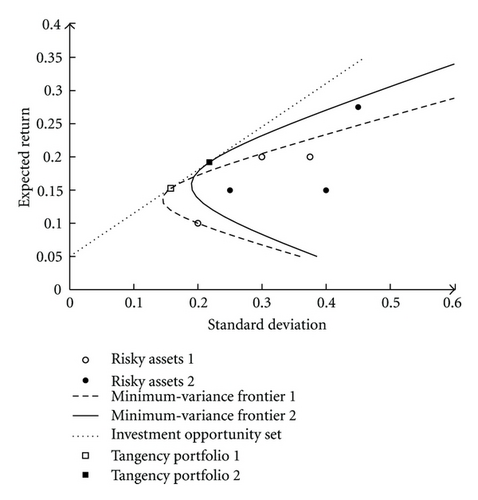
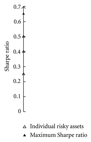
Example 4 (illustration of classical versus alternative characterizations for n = 3). This example illustrates the classical and alternative characterizations of the investment opportunity set in the presence of a risk-free asset. We suppose that the investment universe consists of a risk-free asset which provides the return of 5% and three risky assets that have the following Sharpe ratios: S(x₁) = 0.50, S(x₂) = 0.40, and S(x₃) = 0.25. Given a particular value of a Sharpe ratio, there are infinite combinations of the expected return and standard deviation that produce this Sharpe ratio. For the sake of simplicity, we consider only two sets of risky assets, where each of the risky assets has the same Sharpe ratio as given above. In particular, the first set of parameters for the risky assets is E[x₁] = 20%, σ₁ = 30%, E[x₂] = 20%, σ₂ = 37.5%, E[x₃] = 10%, and σ₃ = 20%. The second set of parameters for the risky assets is E[x₁] = 27.5%, σ₁ = 45%, E[x₂] = 15%, σ₂ = 25%, E[x₃] = 15%, and σ₃ = 40%. The correlation coefficients between the returns of the risky assets are the same in both cases: ρ₁₂ = 0.5 and ρ₂₃ = ρ₃₁ = −0.2.

Figure 2(a) illustrates the classical characterization of the investment opportunity set. This is a two-dimensional standard deviation-expected return space. Observe that in this space the risk-return characteristics of the two sets of risky assets are seemingly different with different minimum-variance frontiers of risky assets and different compositions of the tangency portfolios. However, in both cases the investment opportunity set is the same straight line. Figure 2(b) presents an illustration of the alternative characterization of the investment opportunity set. This is a one-dimensional Sharpe ratio space. In contrast to the classical illustration, the two sets of risky assets fully coincide. The investment opportunity set is represented by the maximum Sharpe ratio.

A natural question to ask is what happens with the investment opportunity set when we change the values of the expected returns and standard deviations of individual risky assets. Will it result in an improvement or worsening of the investment opportunity set? Using the classical characterization of the investment opportunity set, the answer is not clear. A good guess would be the following: if we increase the expected return of a single risky asset while keeping the standard deviation of this asset at the same level, this should improve the investment opportunity set. In contrast, if we increase the standard deviation of a single risky asset while keeping the expected return at the same level, this should worsen the investment opportunity set. But what if we increase both the expected return and standard deviation? An alternative characterization of the investment opportunity set by means of the Sharpe ratios of individual risky assets makes it possible to provide the answer to this question.

To answer this question we need to find the first-order derivatives of the maximum Sharpe ratio with respect to the Sharpe ratios of single risky assets. The vector of partial derivatives of

with respect to S(x_i) is given by

(34)

Intuitively we expect the maximum Sharpe ratio to increase when we increase the Sharpe ratio of a single risky asset in the investment universe. However, this intuition is not always correct. The subsequent theorem characterizes the condition at which this intuition is perfectly correct.

Theorem 2. The sign of the first-order derivative of the maximum Sharpe ratio with respect to the Sharpe ratio of risky asset i coincides with the sign of the weight of risky asset i in the optimal risky portfolio. In particular,

(35)

where sgn (·) is the sign function.

Remark 1. This theorem says that if the weight of risky asset i in the optimal risky portfolio is positive, then an increase in the Sharpe ratio of asset i results in an increase in the maximum Sharpe ratio. Conversely, if the weight of risky asset i in the optimal risky portfolio is negative, then an increase in the Sharpe ratio of asset i results in a decrease in the maximum Sharpe ratio.

Remark 2. If the market is in equilibrium and all risky assets are in positive net supply, then the weights of all risky assets in the market portfolio are positive. Hence, if the market is in equilibrium, then an increase in the Sharpe ratio of any risky asset results in an increase in the maximum Sharpe ratio.

Proof. The vector of partial derivatives of with respect to S(x_i) is given by (34). Observe that is a positive scalar and R⁻¹S is a vector, where each element i is given by

(36)

where R_ji is an element of the cofactor matrix of R. Consequently, the vector of partial derivatives of

with respect to S(x_i) is given by

(37)

The signs of the weights of risky assets in the investor′s optimal risky portfolio (as given by (8)) coincide with the signs of the weights of the risky assets in the tangency portfolio (as given by (15)), that is, sgn (w_i) = sgn (w_ti). Let us write the weights of the risky assets in the tangency portfolio as

(38)

where b = 1/1^′V⁻¹(e − 1r) is a positive scalar; see (14). Then in the proof we will employ the results derived in the proof of Theorem 1. We establish the following:

(39)

We already know how the matrix Σ⁻¹ looks like and the elements of the vector R⁻¹S. This knowledge gives us

(40)

Note that

, det (R) > 0, and σ_i > 0 for all i. Finally observe from (37) that

and from (40) that

. Thus, we conclude that

Example 5 (n = 2). Consider the case where the investment universe consists of two risky assets and a risk-free asset. Suppose that r = 5%, E[x₁] = 9%, σ₁ = 40%, E[x₂] = 20%, σ₂ = 40%, and ρ₁₂ = 0.5. The Sharpe ratios of the assets are S(x₁) = 0.1 and S(x₂) = 0.375. The maximum Sharpe ratio in this case is given by (29) and equals . The weights of the risky assets in the tangency portfolio are w_t1 = −0.3684 and w_t2 = 1.3684. Note that asset 1 is inferior to asset 2 (since asset 1 has a much lower Sharpe ratio as compared to asset 2), the correlation coefficient between the returns on these two assets is rather large, and it is optimal to sell short asset 1.

The computation of the first-order derivatives of the maximum Sharpe ratio with respect to individual Sharpe ratios gives

(41)

Observe that the signs of the first-order derivatives coincide with the signs of the weights. The sign of the first-order derivative of the maximum Sharpe ratio with respect to the Sharpe ratio of the first risky asset is negative which means that an increase in the Sharpe ratio of the first asset results in a decrease in the maximum Sharpe ratio. For the sake of illustration, suppose that the Sharpe ratio of the first asset increases to S(x₁) = 0.2. In this case the maximum Sharpe ratio decreases to

. In contrast, the sign of the first-order derivative of the maximum Sharpe ratio with respect to the Sharpe ratio of the second risky asset is positive which means that an increase in the Sharpe ratio of the second asset results in an increase in the maximum Sharpe ratio. If, for instance, the Sharpe ratio of the second asset increases to S(x₂) = 0.475, the maximum Sharpe ratio increases to

Example 6 (real-world example with n = 15). Considerable academic research documents the benefits of international diversification; see, for example, Grubel [5], Levy and Sarnat [6], and Solnik [7]. The gains from international diversification supposedly stem from relatively low correlations among international stock markets. However, academic research also documents that the average correlation among international stock markets has been increasing over time; see King et al. [8], Longin and Solnik [9], and Goetzmann et al. [10]. Due to the deterioration in diversification opportunities, it is tempting to deduce that the efficiency of international investment has diminished (see, e.g., Eun and Lee [11]). In this example we consider the evolution of the international investment opportunity set through time from the point of view of an investor in the USA. In particular, our goal is to find out whether the efficiency of international investment has really deteriorated.

Our sample of 15 developed markets spans the period from January 1975 to December 2007. The 15 developed markets are Australia, Belgium, France, Germany, Hong Kong, Italy, Japan, the Netherlands, Norway, Singapore, Spain, Sweden, Switzerland, the UK, and the USA. The monthly value-weighted dollar returns for each country are obtained from the data library of Kenneth French (see http://mba.tuck.dartmouth.edu/pages/faculty/ken.french/data_library.html). Monthly risk-free rates of return, proxied by the monthly US T-Bill rates, are obtained from the Ibbotson SBBI 2009 Classic Yearbook. To examine the evolution of the investment opportunity set through time, we divide our overall sample period 1975–2007 into two subperiods: 1975–1991 and 1992–2007.

The maximum Sharpe ratio (computed using either (11) or (17)) of the optimal international portfolio amounts to 0.268 for the first subperiod and to 0.290 for the second subperiod. Yet, consistent with previous findings, the average correlation among international stock markets has increased from 0.466 to 0.581. That is, despite a significant increase in average correlation among stock markets, the investment opportunity set has improved through time, at least for an American investor. Without the knowledge of the alternative characterization of the maximum Sharpe ratio, all we can say is that the improvement of the investment opportunity set has been caused by some favorable changes in the excess returns and standard deviations of returns on international stock markets. The knowledge of the alternative characterization of the maximum Sharpe ratio motivates us to investigate the changes in the average Sharpe ratio. We find that the average Sharpe ratio of international stock markets has increased from 0.126 to 0.148. Thus, whereas the increased correlations have exerted a negative impact, the increased Sharpe ratios have exerted a positive impact on the investment opportunity set. The combined effect of both the increased correlations and increased Sharpe ratios has exerted a positive impact on the efficiency of international investment.

At the end of this example we would like to emphasize the advantage (in the investment practice) of using Sharpe ratios and correlations to describe the investment opportunity set. In particular, this example convincingly demonstrates that it is not enough to examine only the changes in diversification opportunities in order to deduce the changes in the investment opportunity set. One also needs to study the changes in the Sharpe ratios in order to have a complete picture of the evolution of the investment opportunity set.

4. The CAPM Relationship Reconsidered

So far we have reconsidered some results of the Markowitz portfolio theory in the presence of a risk-free asset. The classical CAPM is, in fact, none other than the Markowitz portfolio theory in the presence of a risk-free asset paired with an equilibrium condition. Therefore, it is pretty straightforward to reconsider the CAPM relationship in terms of Sharpe ratios.

The standard CAPM (expected return-beta) relationship is as follows:

(42)

where x_M is the return on the market portfolio and β_i is given by

(43)

where ρ_i is the correlation coefficient between the returns on asset i and the market portfolio and σ_M is the standard deviation of returns on the market portfolio. The CAPM relationship can be rewritten as

(44)

that is, as the Sharpe ratio-rho relationship

(45)

This says that in equilibrium the Sharpe ratio of risky asset i equals the Sharpe ratio of the market portfolio times the correlation coefficient between the returns on asset i and the market portfolio. The Sharpe ratio is often alternatively called the price of risk. Thus, yet another formulation of the CAPM relationship could be the following: in equilibrium the price of risk of asset i equals the market price of risk times the correlation coefficient between the returns on asset i and the market. If ρ_i = 0, then S(x_i) = 0, which means that there is no risk to be priced. The higher the correlation coefficient ρ_i, the higher the Sharpe ratio S(x_i). Since ρ_i ≤ 1, we conclude that S(x_i) ≤ S(x_M). That is, the Sharpe ratio of the market portfolio is the maximum Sharpe ratio.

The difference between the actual and equilibrium expected rates of return on risky asset i is denoted by (Jensen′s) alpha:

(46)

Jensen′s alpha is one of the most popular portfolio performance measures used in practice. However, it is widely known now that Jensen′s alpha has one serious drawback. Namely, if α(x_i) > 0, then the value of alpha can be manipulated by leverage (see, e.g., Ingersoll et al. [12]). In particular, by borrowing money at the risk-free rate one can create an asset with return y_i = a(x_i − r) + r, a > 1. It is easy to check that α(y_i) = aα(x_i) > α(x_i). That is, alpha can in theory be made as large as desirable by leverage. The problem with Jensen′s alpha stems from the fact that alpha is the abnormal return unadjusted for risk.

To mitigate the leverage problem inherent in alpha one can employ the Treynor ratio (see Treynor [13]). However, there is another way around the leverage problem. Divide the left- and right-hand sides of (46) by σ_i. Then we obtain

(47)

We will refer to α^′(x_i) = α(x_i)/σ_i as the adjusted Jensen′s alpha. The adjusted Jensen′s alpha is easy to interpret: it is the abnormal return adjusted for risk, or the abnormal Sharpe ratio. The form of the adjusted Jensen′s alpha resembles the form of the information ratio (also known as the appraisal ratio or the Treynor-Black ratio; see Treynor and Black [14]). However, whereas in the information ratio the Jensen′s alpha is divided by the nonsystematic risk, in the adjusted version the Jensen′s alpha is divided by the total risk. One can easily check that, for any a > 0, α^′(y_i) = α^′(x_i), so the adjusted Jensen′s alpha cannot be manipulated by leverage.

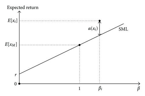
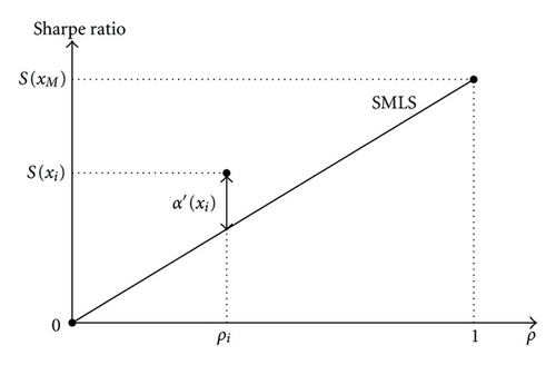
Figure 3(a) presents the classical illustration of the CAPM relationship. This is a beta-expected return space. SML denotes the security market line. It is a straight line with intercept r and slope E[x_M] − r. If the market is in equilibrium, all assets should lie along the security market line. Figure 3(b) presents an alternative illustration of the CAPM relationship. This is a rho-Sharpe ratio space. SMLS denotes the security market line segment. It is a part of a straight line with zero intercept and slope S(x_M). If the market is in equilibrium, all assets should lie along the security market line segment. Figure 3 also demonstrates the values of the Jensen′s alpha and the adjusted Jensen′s alpha for asset i which provides abnormal return.

5. Summary

In this paper we showed that in the presence of a risk-free asset the investment opportunity set can be characterized in terms of the vector of the Sharpe ratios of risky assets and the correlation matrix. Consequently, this implies that the changes in the risk-return characteristics of individual risky assets that preserve the Sharpe ratios and the correlation matrix do not change the investment opportunity set. We performed the comparative static analysis which provides a simple answer to the question of what happens with the investment opportunity set when we change the characteristics of individual risky assets. We demonstrated the advantages of using the alternative characterization of the investment opportunity set in the investment practice. Using the Sharpe ratio thinking we reconsidered the CAPM relationship and proposed how to adjust the Jensen′s alpha in order to properly measure abnormal portfolio performance.

Acknowledgment

The author is grateful to Steen Koekebakker and the anonymous referees for their comments.

References

1 Markowitz H. M., Portfolio selection, Journal of Finance. (1952) 7, 77–91.
10.1111/j.1540-6261.1952.tb01525.x
Web of Science® Google Scholar
2 Merton R. C., An analytic derivation of the efficient portfolio frontier, Journal of Financial and Quantitative Analysis. (1972) 7, 1851–1872.
10.2307/2329621
Web of Science® Google Scholar
3 Roll R., A critique of the asset pricing theory′s tests part I: on past and potential testability of the theory, Journal of Financial Economics. (1977) 4, no. 2, 129–176, 2-s2.0-0039473752.
10.1016/0304-405X(77)90009-5
Web of Science® Google Scholar
4 Huang C. f. and Litzenberger R. H., Foundations for Financial Economics, 1993, Prentice Hall, Englewood Cliffs, NJ, USA.
Google Scholar
5 Grubel H. G., Internationally diversified portfolios: welfare gains and capital flows, American Economic Review. (1968) 58, no. 5, 1299–1314.
Web of Science® Google Scholar
6 Levy H. and Sarnat M., International diversification of investment portfolios, American Economic Review. (1970) 60, no. 4, 668–675.
Web of Science® Google Scholar
7 Solnik B. H., Why not diversify internationally rather than domestically?, Financial Analysts Journal. (1974) 30, no. 4, 48–54.
10.2469/faj.v30.n4.48
Google Scholar
8 King M., Sentana E., and Wadhwani S., Volatility and links between national stock markets, Econometrica. (1994) 62, no. 4, 901–933.
10.2307/2951737
Web of Science® Google Scholar
9 Longin F. and Solnik B., Is the correlation in international equity returns constant: 1960–1990?, Journal of International Money and Finance. (1995) 14, no. 1, 3–26, 2-s2.0-0002525307.
10.1016/0261-5606(94)00001-H
Web of Science® Google Scholar
10 Goetzmann W. N., Li L., and Rouwenhorst K. G., Long-term global market correlations, Journal of Business. (2005) 78, no. 1, 1–38, 2-s2.0-17644378119, https://doi.org/10.1086/426518.
10.1086/426518
Web of Science® Google Scholar
11 Eun C. S. and Lee J., Mean-variance convergence around the world, Journal of Banking and Finance. (2010) 34, no. 4, 856–870, 2-s2.0-76049098695, https://doi.org/10.1016/j.jbankfin.2009.09.016.
10.1016/j.jbankfin.2009.09.016
Web of Science® Google Scholar
12 Ingersoll J., Spiegel M., and Goetzmann W., Portfolio performance manipulation and manipulation-proof performance measures, Review of Financial Studies. (2007) 20, no. 5, 1503–1546, 2-s2.0-34548532494, https://doi.org/10.1093/rfs/hhm025.
10.1093/rfs/hhm025
Web of Science® Google Scholar
13 Treynor J. L., How to rate management investment funds, Harvard Busines Review. (1966) 43, 63–75.
Web of Science® Google Scholar
14 Treynor J. L. and Black F., How to use security analysis to improve portfolio selection, Journal of Business. (1973) 46, no. 1, 66–86.
10.1086/295508
Web of Science® Google Scholar

Citing Literature

All articles

Sharpe (Ratio) Thinking about the Investment Opportunity Set and CAPM Relationship

Abstract

1. Introduction

2. The Maximum Sharpe Ratio

3. Alternative Characterization of the Maximum Sharpe Ratio

4. The CAPM Relationship Reconsidered

5. Summary

Acknowledgment

References

Citing Literature

Figures

References

Information

About Wiley Online Library

Help & Support

Opportunities

Connect with Wiley

Sharpe (Ratio) Thinking about the Investment Opportunity Set and CAPM Relationship

Abstract

1. Introduction

2. The Maximum Sharpe Ratio

3. Alternative Characterization of the Maximum Sharpe Ratio

4. The CAPM Relationship Reconsidered

5. Summary

Acknowledgment

References

Citing Literature

Figures

References

Related

Information