The standard estimate of prevalence is the proportion of positive results obtained from the application of a diagnostic test to a random sample of individuals drawn from the population of interest. When the diagnostic test is imperfect, this estimate is biased. We give simple formulae, previously described by Greenland (1996) for correcting the bias and for calculating confidence intervals for the prevalence when the sensitivity and specificity of the test are known. We suggest a Bayesian method for constructing credible intervals for the prevalence when sensitivity and specificity are unknown. We provide R code to implement the method.

1. Introduction

The prevalence, θ, of a disease is the proportion of subjects in the population of interest who have the disease in question [1, page 46]. A standard way to estimate prevalence is to apply a diagnostic test to a random sample of n individuals and use the estimator

()

where T is the number of individuals who test positive.

The sensitivity, se, of a diagnostic test for presence/absence of a disease is the probability that the test will give a positive result, conditional on the subject being tested having the disease, whilst the specificity, sp, is the probability that the test will give a negative result, conditional on the subject not having the disease. An imperfect test is one for which at least one of se and sp is less than one. An imperfect test may give either or both of a false positive or a false negative result, with respective probabilities 1 − sp and 1 − se. A similar issue arises in individual diagnostic testing. In that context, prevalence is assumed to be known and the objective is to make a diagnosis for each subject tested. Important quantities are then the positive and negative predictive values, defined as the conditional probabilities that a subject does or does not have the disease in question, given that they show a positive or negative test result, respectively. Even when both se and sp are close to one, the positive and negative predictive values of a diagnostic test depend critically on the true prevalence of the disease in the population being tested. In particular, for a rare disease, the positive predictive value can be much smaller than either se or sp.

2. Estimation of Prevalence

Suppose that an imperfect test is applied to a random sample of n subjects, T of whom give a positive result. The standard estimator

given by (1) is now biased for θ. Let ϕ denote the expectation of

. Then, the relationship between θ and ϕ is linear, and given by

()

[2]. Under the reasonable assumption that se + sp > 1, that is, that the test is superior to the toss of a coin and ϕ is an increasing function of θ. It follows that if the values of se and sp are known a confidence interval, (a, b) say, for ϕ can be converted straightforwardly to a confidence interval (c, d) for θ by applying the pair of transformations

()

See Figure 1 for an illustration.

Details are in the caption following the image — **Figure 1**
Open in figure viewer PowerPoint

Converting an interval estimate of ϕ, the probability of a positive test result, into an interval estimate of θ, the true prevalence, for a test with sensitivity 0.9 and specificity 0.75. The vertical and horizontal arrows denote the interval estimates of ϕ and θ, respectively.

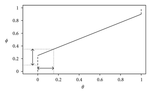
Typically, when the true prevalence is low, ϕ > θ and the effect of the bias correction is to shift the interval estimate of prevalence towards lower values. For example, if se = sp = 0.9 and θ = 0.01, then ϕ = 0.108. As the true prevalence increases, the relative difference between ϕ and θ decreases; for example, if se = sp = 0.9 as before but now θ = 0.2, then ϕ = 0.26.

3. Unknown Sensitivity and Specificity

If se and sp are unknown, θ can still be estimated, albeit with reduced precision, using a Bayesian approach. This requires us to specify a prior distribution for θ and informative prior distributions for se and sp (informative, because the data give essentially no information about se or sp). Assume temporarily that se and sp are both known. The sampling distribution of T, the number of positive test results out of n individuals tested, given θ is binomial, with number of trials n and probability of a positive outcome ϕ = c₁ + c₂θ, where c₁ = 1 − sp and c₂ = se + sp − 1. A convenient, uninformative prior for θ is the uniform distribution on (0,1). The marginal distribution of T is then obtained as

()

where

()

is the incomplete beta function. The posterior distribution for θ given se and sp follows as

()

where h(t) is given by (4). Finally, to allow for the uncertainty in se and sp, we substitute c₁ = 1 − sp and c₂ = se + sp − 1 on the right-hand-side of (6) and integrate with respect to the joint prior, p(u, v) say, for se and sp, to give the posterior distribution for θ as

()

4. Example

Suppose that we sample n = 100 individuals, of whom T = 20 give positive results. The uncorrected estimate of prevalence (1) is 0.2. Solving the quadratic equation (0.2−θ)² = 1.96²θ(1 − θ) gives a 95% confidence interval for θ as (0.122,0.278). If we assume that se = sp = 0.9, inversion of (2) gives the corrected estimate , whilst (3) gives the corresponding 95% confidence interval as (0.042,0.236).

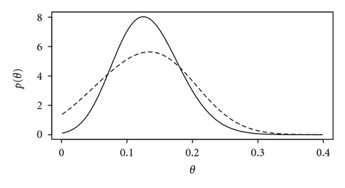
We now assume that se and sp are unknown and specify independent beta prior distributions, each with parameters α = β = 2 but scaled to lie in the interval (0.8,1); hence, the prior for each of se and sp is unimodal wit prior expectation 0.9. A 95% Bayesian credible interval for θ is (0.003,0.246), wider than and shifted to the left of the classical confidence interval. Incidentally, the corresponding 95% Bayesian credible interval for θ assuming known se = sp = 0.9 is (0.038,0.230). This is much closer to the classical confidence interval, which is as expected since we have specified an uninformative prior for θ. Figure 2 shows the posterior distributions for θ assuming known or unknown se and sp. The greater spread of the latter represents the loss of precision that results from not knowing the sensitivity and specificity of the test.

5. Discussion

When both se and sp are close to one, the absolute bias of the uncorrected estimator defined in (1) is small but the relative bias may still be substantial. Also, in some settings, practical constraints dictate the use of tests with relatively low sensitivity and/or specificity. An example is the use by the African Programme for Onchocerciasis Control of a questionnaire-based assessment of community-level prevalence of Loa loa in place of the more accurate, but also more expensive and invasive, finger-prick blood-sampling and microscopic detection of microfilariae [3].

The simple method described here to take account of known sensitivity and/or specificity less than one is rarely described explicitly in epidemiology text books. For example, [4, Section 4.2] note that it is “possible to correct for biases… due to the use of a nonspecific diagnostic test” but give no details, perhaps because their focus is on comparing efficacies of different treatments rather than on estimating prevalence.

Exactly the same argument would apply to the estimation of prevalence in more complex settings. For example, where prevalence is modelled as a function of explanatory variables, say θ = θ(x), an interval estimate for θ(x) can be calculated at each value of x by applying (3) to the corresponding interval estimate of ϕ(x).

The Bayesian method for dealing with unknown se and sp does not yield explicit formulae for point or interval estimates of prevalence, but the required computations are not burdensome; an R function is listed in the Algorithm and can be downloaded from the author′s web-site (http://www.lancs.ac.uk/staff/diggle/prevalence-estimation.R/).

Algorithm 1: R code.

#
# R function for Bayesian estimation of prevalence using an
# imperfect test.
#
# Notes
#
# 1. Prior for prevalence is uniform on (0,1)
# 2. Priors for sensitivity and specificity are independent scaled
# beta distributions
# 3. Function uses a simple quadrature algorithm with number of
# quadrature points as an optional argument "ngrid" (see below);
# the default value ngrid=20 has been sufficient for all examples
# tried by the author, but is not guaranteed to give accurate
# results for all possible values of the other arguments.
#
prevalence.bayes<-function(theta,T,n,lowse=0.5,highse=1.0,
sea=1,seb=1,lowsp=0.5,highsp=1.0,spa=1,spb=1,ngrid=20,coverage=0.95) {
#
# arguments
# theta: vector of prevalences for which posterior density is required
# (will be converted internally to increasing sequence of equally
# spaced values, see "result" below)
# T: number of positive test results
# n: number of indiviudals tested
# lowse: lower limit of prior for sensitivity
# highse: upper limit of prior for sensitivity
# sea,seb: parameters of scaled beta prior for sensitivity
# lowsp: lower limit of prior for specificity
# highsp: upper limit of prior for specificity
# spa,spb: parameters of scaled beta prior for specificity
# ngrid: number of grid-cells in each dimension for quadrature
# coverage: required coverage of posterior credible interval
# (warning message given if not achieveable)
#
# result is a list with components
# theta: vector of prevalences for which posterior density has
# been calculated
# post: vector of posterior densities
# mode: posterior mode
# interval: maximum a posteriori credible interval
# coverage: achieved coverage
#
ibeta<-function(x,a,b) {
pbeta(x,a,b)*beta(a,b)
}
ntheta<-length(theta)
bin.width<-(theta[ntheta]-theta[1])/(ntheta-1)
theta<-theta[1]+bin.width*(0:(ntheta-1))
integrand<-array(0,c(ntheta,ngrid,ngrid))
h1<-(highse-lowse)/ngrid
h2<-(highsp-lowsp)/ngrid
for (i in 1:ngrid) {
se<-lowse+h1*(i-0.5)
pse<-(1/(highse-lowse))*dbeta((se-lowse)/(highse-lowse),sea,seb)
for (j in 1:ngrid) {
sp<-lowsp+h2*(j-0.5)
psp<-(1/(highsp-lowsp))*dbeta((sp-lowsp)/(highsp-lowsp),spa,spb)
c1<-1-sp
c2<-se+sp-1
f<-(1/c2)*choose(n,T)*(ibeta(c1+c2,T+1,n-T+1)-ibeta(c1,T+1,n-T+1))
p<-c1+c2*theta
density<-rep(0,ntheta)
for (k in 1:ntheta) {
density[k]<-dbinom(T,n,p[k])/f
}
integrand[,i,j]<-density*pse*psp
}
}
post<-rep(0,ntheta)
for (i in 1:ntheta) {
post[i]<-h1*h2*sum(integrand[i,,])
}
ord<-order(post,decreasing=T)
mode<-theta[ord[1]]
take<-NULL
prob<-0
i<-0
while ((prob<coverage/bin.width)&(i<ntheta)) {
i<-i+1
take<-c(take,ord[i])
prob<-prob+post[ord[i]]
}
if (i==ntheta) {
print("WARNING: range of values of theta too narrow")
}
interval<-theta[range(take)]
list(theta=theta,post=post,mode=mode,interval=interval,coverage=prob*bin.width)
}
#
# example
#
n<-100
T<-20
ngrid<-25
lowse<-0.7
highse<-0.95
lowsp<-0.8
highsp<-1.0
sea<-2
seb<-2
spa<-4
spb<-6
theta<-0.001*(1:400)
coverage<-0.9
result<-prevalence.bayes(theta,T,n,lowse,highse,
sea,seb,lowsp,highsp,spa,spb,ngrid,coverage)
result$mode # 0.115
result$interval # 0.011 0.226
plot(result$theta,result$post,type="l",xlab="theta",ylab="p(theta)")

Appendix

For more details, see Algorithm 1.

References

Citing Literature

All articles

Estimating Prevalence Using an Imperfect Test

Abstract

1. Introduction

2. Estimation of Prevalence

3. Unknown Sensitivity and Specificity

4. Example

5. Discussion

Appendix

References

Citing Literature

Figures

References

Information

About Wiley Online Library

Help & Support

Opportunities

Connect with Wiley

Estimating Prevalence Using an Imperfect Test

Abstract

1. Introduction

2. Estimation of Prevalence

3. Unknown Sensitivity and Specificity

4. Example

5. Discussion

Appendix

References

Citing Literature

Figures

References

Related

Information