The Generalized PSO: A New Door to PSO Evolution
Abstract
A generalized form of the particle swarm optimization (PSO) algorithm is presented. Generalized PSO (GPSO) is derived from a continuous version of PSO adopting a time step different than the unit. Generalized continuous particle swarm optimizations are compared in terms of attenuation and oscillation. The deterministic and stochastic stability regions and their respective asymptotic velocities of convergence are analyzed as a function of the time step and the GPSO parameters. The sampling distribution of the GPSO algorithm helps to study the effect of stochasticity on the stability of trajectories. The stability regions for the second-, third-, and fourth-order moments depend on inertia, local, and global accelerations and the time step and are inside of the deterministic stability region for the same time step. We prove that stability regions are the same under stagnation and with a moving center of attraction. Properties of the second-order moments variance and covariance serve to propose some promising parameter sets. High variance and temporal uncorrelation improve the exploration task while solving ill-posed inverse problems. Finally, a comparison is made between PSO and GPSO by means of numerical experiments using well-known benchmark functions with two types of ill-posedness commonly found in inverse problems: the Rosenbrock and the “elongated” DeJong functions (global minimum located in a very flat area), and the Griewank function (global minimum surrounded by multiple minima). Numerical simulations support the results provided by theoretical analysis. Based on these results, two variants of Generalized PSO algorithm are proposed, improving the convergence and the exploration task while solving real applications of inverse problems.
1. Introduction
Particle swarm optimization (PSO) is an evolutionary computation technique [1] for optimization which is inspired by the social behavior of individuals in groups in nature. The particle swarm algorithm applied to optimization problems is very simple.
(1)Individuals, or particles, are represented by vectors whose length is the number of degrees of freedom of the optimization problem.
(2) To start, a population of particles is initialized with random positions () and velocities (). A misfit or cost function is evaluated for each particle.
Convergence properties and PSO trajectories were analyzed, and helped to clarify some numerical aspects of the PSO algorithm; see [2–6]. Also, based on these analysis, some parameter selection strategies were proposed (see, e.g., [5]).
Physical analogy with a damped mass-spring oscillator was introduced by Brandstätter and Baumgartner [8] to optimize electrical engineering problems, nevertheless, this analogy was not completely exploited in their work. Recently, Fernández Martínez et al. [9] used this analogy to derive the PSO continuous model and to present a systematic study of PSO trajectories by means of stability analysis of the deterministic PSO difference equations involved and fixed point techniques. The PSO convergence can then be explained in terms of some combined criteria: trajectory attenuation, trajectory oscillation, and center attraction potential, explaining the success in achieving convergence of some parameter sets found in the literature.
Interdisciplinary approaches, from classical Newtonian mechanics to molecular dynamics theory, have been recently proposed by Mikki and Kishk [10] to study the thermodynamic behavior of PSO, providing new criterion to analyze the algorithm convergence. Also, stagnation analysis [11] and statistical approaches [12] were used to characterize the sampling distribution of PSO in presence of stochasticity and to provide criteria for the PSO parameter selection.
In this paper, we present a generalized form of the particle swarm optimization (PSO), which is derived from a continuous version of PSO. This idea has been partially presented in [9, 10, 13], but in this manuscript is fully developed.
(1) The deterministic and stochastic stability regions and the asymptotic velocities of convergence of the GPSO algorithm are analyzed as a function of the time step, the local and global accelerations, and the inertia value.
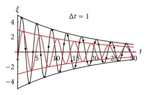
(2) Generalized and continuous PSO models are compared in terms of attenuation and oscillation properties as a function of the time step and the PSO parameters. As expected, GPSO properties tend to those of the continuous PSO model, as the time step goes to zero.
(3) The sampling distribution of the GPSO algorithm is also analyzed and helps to study the effect of stochasticity on the stability of trajectories. The stability region for the second-, third-, and fourth-order moments depends on inertia, local, and global accelerations and time discretization step. These regions are smaller in size than the corresponding deterministic stability region for the same time step. Regions increase in size as time step decreases. Also, for a given time step, the maximum size of the second-order stability region occurs when local and global accelerations are equal. Properties of the second-order moments—variance, covariance, variogram, and correlogram—are also explored with a moving center of attraction, assuming that l(t) and g(t) exhibit a deterministic behavior. This analysis serve to propose some promising parameter sets. High variance and temporal uncorrelation improve the exploration task needed to solve ill-posed inverse problems. A similar idea has been also proposed by Clerc [11] under stagnation.
(4) Finally, a comparison is made between PSO and the GPSO by means of numerical experiments using well-known benchmark functions supporting the theoretical results. Based on these results two variants of generalized PSO algorithm are proposed, improving the convergence and the exploration task while solving real applications in inverse problems modeling.
2. The Pso Difference Equations
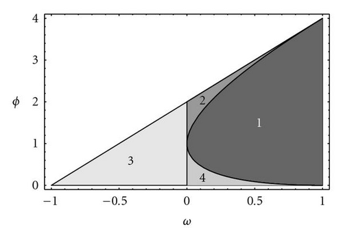
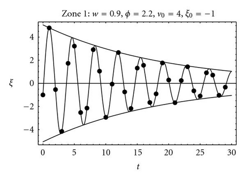
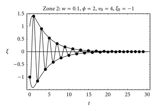
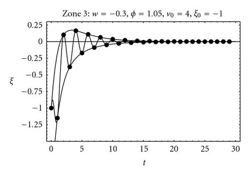
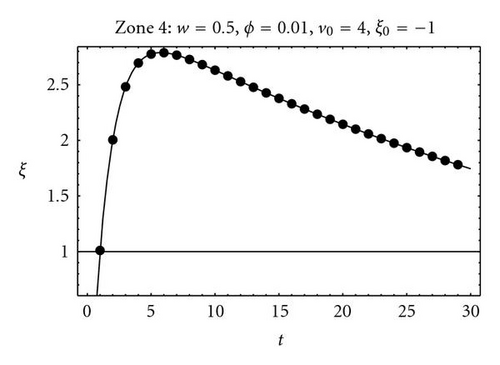
Let us introduce the PSO deterministic case which is modeled by difference equation (7) and ϕ is in this case is a real constant. As we will show on the stochastic stability analysis, this model describes the mean behavior of random trajectories, , when is in this case the average value of random variable ϕ.
3. The Pso Continuous Model
The PSO differential model (15) has been deduced from a mechanical analogy [9]: a damped mass-spring system of unit mass, damping factor, b = 1 − w, and stiffness constant, k = ϕ. The knowledge of the trajectories of both the continuous and the discrete model helped to explain why some zones of the parameter space (w,ϕ) provide better convergence, in terms of some combined criteria: trajectory attenuation, trajectory oscillation, and center attraction potential. The same conclusions are true for the GPSO as it will be demonstrated.
4. The Generalized Pso
The idea we propose here is to generalize the PSO algorithm for any time step, Δt. Without loss of generality, the theoretical development is done in one dimension, as if we were reasoning separately for each particle coordinate.
4.1. GPSO deterministic stability analysis
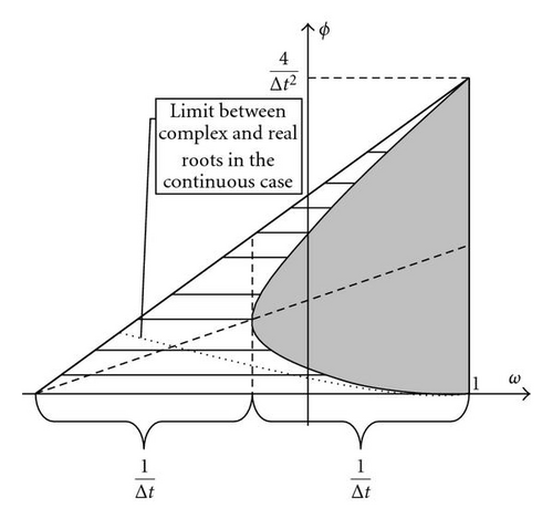
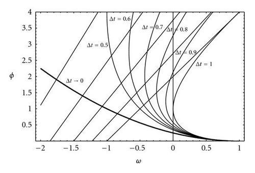
This approach allows us also to calculate the deterministic stability region of the generalized PSO.
4.1.1. Stagnation case
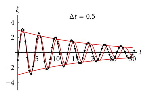
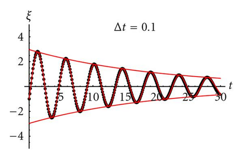
4.1.2. Moving center of attraction
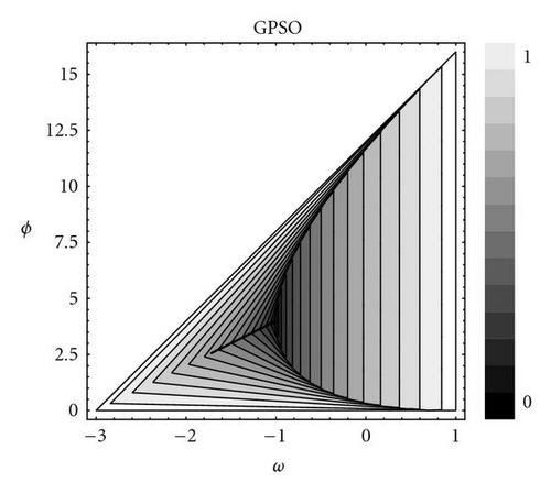
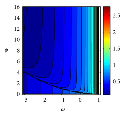
Figure 5 shows the deterministic spectral radius—associated to the asymptotic velocity of convergence—for the generalized PSO. The similarity with the PSO case (Δt = 1) is absolute, and the black zone of high velocity increases in size. The asymptotic velocity tends to infinite on the parabola vertex, (1 − 1/Δt, 1/Δt2).

5. Some Interesting Properties of The Gpso
With GPSO, we have performed a numerical analysis that seeks to explain why some pairs of (w,ϕ) in certain zones of the deterministic convergence triangle work in achieving convergence and why others do not.
5.1. Center attraction
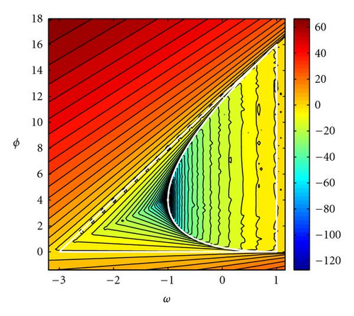
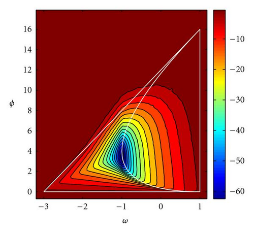
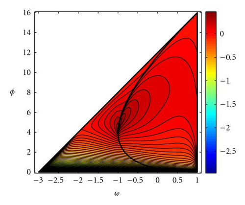
For a GPSO simplified model where , without objective function, two tests have been made: one deterministic (Figure 6(a)) and the other using random ϕ parameters (Figure 6(b)).
For the deterministic one,
- (1)
100 particles, are randomly initialized over the two dimensional domain [−100,100] × [−100,100];
- (2)
a parameter grid (ω,ϕ) is defined over the region (ω,ϕ) ∈ [−3,1] × [0,18] with the following grid steps: Δw = 0.06, Δϕ = 0.02;
- (3)
each particle ξp=(xp,yp) follows the simplified trajectory:
()for each point (ω,ϕ) of the parameter grid; - (4)
for each (ω,ϕ), the particle nearest to the attractor point—(0,0) in this case—is found after 100 iterations. Its distance to the attractor point, dmin (ω,ϕ), is calculated and expressed in logarithmic scale;
- (5)
The contour map log dmin (ω,ϕ) is plotted over the parameter region [−3,1] × [0,18].
In the random case, the same test has been performed, but 300 simulations have been made for each (ω,ϕ) (instead of only one simulation in the deterministic case) and the median of dmin (ω,ϕ) has been computed. It can be observed that in the upper-right zone of the convergence triangle there is no convergence (Figure 6(b)). This is due to the high amplitudes and frequencies of the trajectories in this zone.
5.2. Comparison to the PSO continuous model
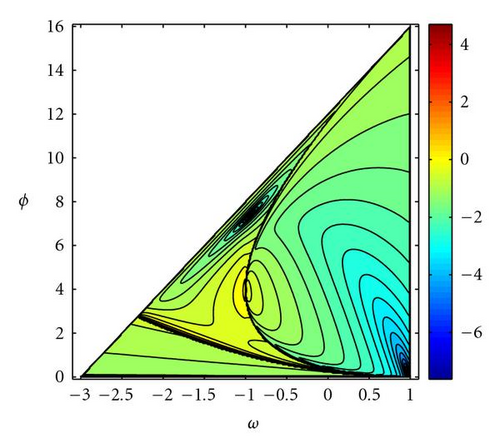
It has been observed that in zones of optimal convergence, the continuous and discrete trajectories differ a little [9]. Figure 7 shows the relative logarithmic misfit between the GPSO for Δt = 0.5 and the PSO continuous model, both using their trajectories and/or their respective envelope curves. It can be observed that as Δt decreases, the size of the zone of similarity increases. The PSO stability triangle is embedded in this zone.
5.3. Attenuation and oscillation
No convergence close to the point (w,ϕ) = (1 − 1/Δt,1/Δt2), vertex of the parabola, can be explained by the quick attenuation of the trajectories amplitude and fast convergence to the oscillation center, that in the first moments of the application of the algorithm is usually far from the optimum. Figure 8 shows, for different (w,ϕ) points on the stability region, the number of iterations (expressed in logarithmic scale) needed to reduce the amplitude of the GPSO trajectories in 90% for Δt = 0.5, and the comparison to PSO and to the continuous case. As in the previous figure, similarity with the continuous increases as Δt → 0.
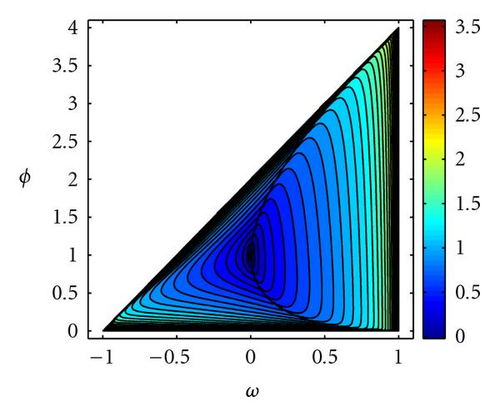
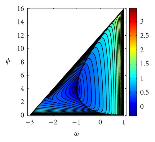
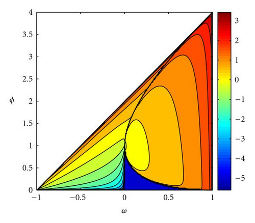
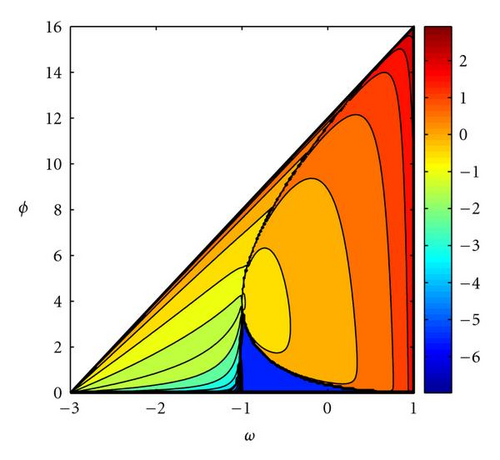
The area between envelopes for the discrete trajectories has been used as a measure of the exploratory capacity of the PSO. It can be seen that it is higher as w increases in the complex zone and near to the upper convergence limit in the real zone. Figure 9 shows the area between envelope curves for the GPSO with Δt = 0.5 and its comparison to the PSO case. These two last magnitudes (attenuation and oscillation) have been proposed as measures of the exploration capabilities associated to the deterministic PSO trajectories [9].
6. The Sampling Distribution of The Gpso Algorithm
In this section, we analyze the effect of stochasticity on the stability of GPSO trajectories using the methodology first proposed by Poli [12]. Trajectories are modeled as stochastic processes whose univariate and bivariate statistical moments must satisfy the PSO difference equations involved. The methodology consists in discretizing the PSO continuous model (15) and applying fixed point analysis to the dynamical systems deduced for the first- to fourth-order moments describing the trajectories stability. This analysis is performed under stagnation and with a moving center of attraction. We show that the stability regions are the same in both cases.
6.1. Stagnation case
6.1.1. First- and second-order moments
(1) Stability of the first-order moments only involves the matrix , and logically provides the same results as GPSO deterministic stability analysis.
Figure 10 shows the contour lines of the spectral radius of the stochastic iteration matrix on the unit circle for Δt = 0.5 and α = 1. As it can be observed, the isolines bend on their upper part, remembering the results shown in Figure 6(b).
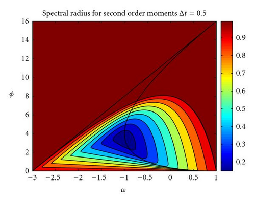
Finally, the second-order stability region increases its size as Δt diminishes. Besides, GPSO algorithm with Δt > 1 introduces for the same (w,ϕ) a higher variance on the trajectories.
The same methodology can be applied to determine the skewness and kurtosis stability regions. Results are presented for a moving center of attraction.
6.2. Moving center of attraction
One can show the following.
(1) The stochastic stability region for the first- and second-order moments is the same that in case of stagnation.
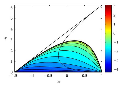
(3) The variance increases its value from 0 in until +∞ on the stochastic border line. Isolines are shown in Figure 11(a). Variance is also null for α = 2 (al = 0), α = 0 (ag = 0).
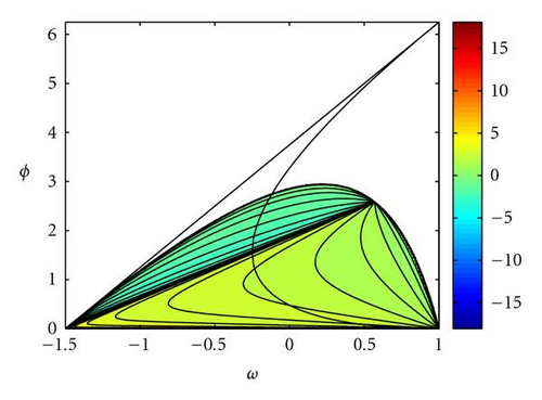
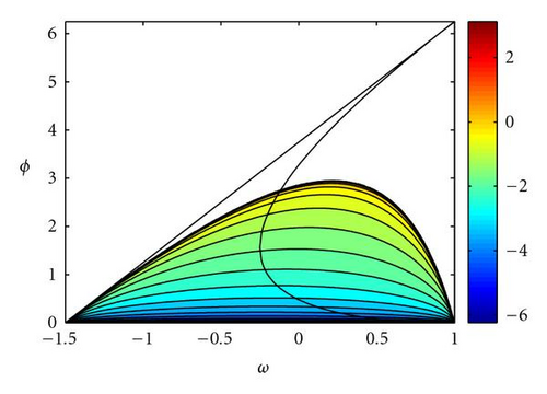
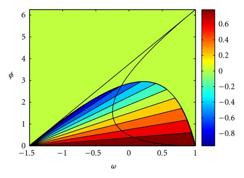
(4) The covariance is zero in and in the line , which is one of the median of the deterministic stability triangle. Covariance is negative above this line. Figure 11(b) shows the contour plot of sgn(Cov) · |ln |Cov||⋅ Covariance is also null for any Δt if al = 0 or ag = 0.
for any point on the stability region of the second-order moments, and does not depend on α, neither on the local and global best trajectories. Correlation coefficient is 1 in and is null on the line Isolines are straight lines passing in (w,ϕ) = (1 − 2/Δt,0) (Figure 11(d)).
6.2.1. Skewness
Our analysis provides the following results.
- (i)
The region where the skewness fix point exists coincides with the region of stability of the second-order moments, nevertheless, the region of skewness stability (where the fixed point is correctly approximated by the iterative PSO algorithm) is smaller in size than the region of second-order stability. Both regions coincide for many w values on (−1,1). This result has been also pointed by Poli [12] in the PSO case, for inertia values restricted to the interval [0,1]. Also, the region of skewness stability tends to the region of second-order stability as time step, Δt, goes to zero.
- (ii)
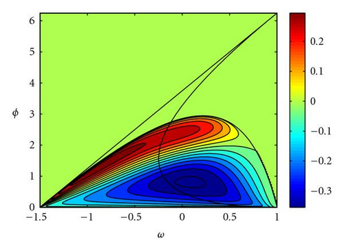
Skewness is null for any Δt if α = 1 (ag = al). Skewness is positive in the upper zone under the second-order stability hyperbola for α < 1 (ag < al), and negative in the bottom zone. For α > 1 (ag > al) the sign swaps between these two zones for any Δt (Figure 12(a)). Skewness does only depend on the sign of g(tp) − l(tp) but not on its absolute value.
6.2.2. Kurtosis
Kurtosis stability analysis involves a linear system with ℝ14 × ℝ14 iteration matrix.
The main results are the following.
- (i)
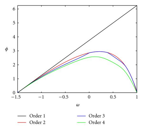
The regions of orders 1, 2, 3, and 4 are nested, being the region of kurtosis stability the smallest on size (Figure 12(b)). This imply that while mean, variance, covariance, and skewness are stable, the kurtosis grows indefinitely. This last result has been also pointed by [12] in the PSO case under stagnation.
- (ii)
All these regions of stability tend to coincide as Δt decreases (GPSO case with Δt < 1). In the limit (Δt → 0), they tend to the continuous stability region (33).
7. Numerical Experiments on Benchmark Functions
To confirm the above-mentioned theoretical results, we ran several numerical experiments on benchmark functions with two types of ill-posedness commonly found in inverse problems: the Rosenbrock and the “elongated” DeJong functions (global minimum located in a very flat area), and the Griewank function (global minimum surrounded by multiple minima). A similar analysis has been done in [9] for the PSO case, showing that as the ill-posedness increases, PSO parameters from the complex stability region, with inertia values from 0.5 to 0.9, and medium to high total accelerations seem to give systematically very good results. Also, in case of cost functions with multiple local minima, the real stability zone of negative inertia values (around −0.55) and total acceleration from 0.6 to 1.2 give very good performance with respect to the percentage of success.
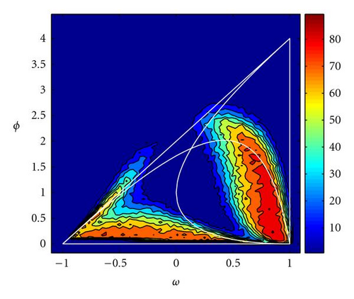
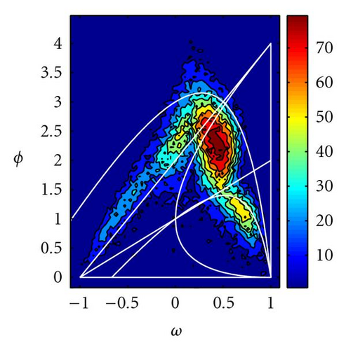
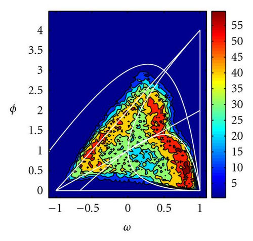
Figure 13 shows the percentage of times (over 100 simulations) that PSO and GPSO (with Δt = 0.5) arrive very close (within a tolerance of 10−5) to the global optimum after 100 iterations. It can be observed that the convergence zone increases in size and the best parameters move towards decreasing inertia values and increasing accelerations, confirming our previous theoretical analysis. Good parameter sets are close to the limit of stochastic stability region (hyperbola (44)). Only for the elongated DeJong function good parameter sets are partly above this line. This parameter region has also been pointed by Clerc [11] in the PSO case, under the stagnation hypothesis, and only for positive inertia values.
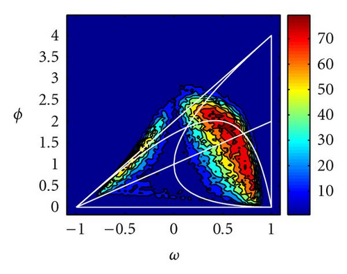
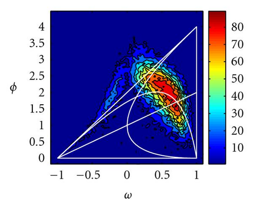
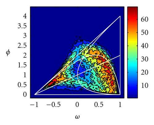
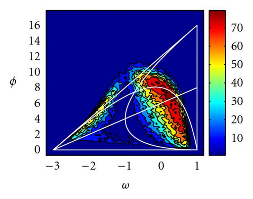
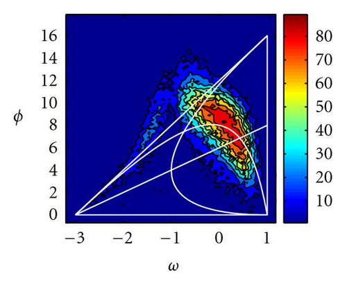
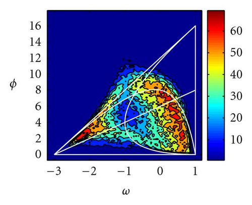
For the Griewank function parameters between the median of the deterministic triangle and the hyperbola (44), and inertia values around −0.5 (in the PSO case) give also a very good performance. In the GPSO case, the inertia values are shifted −1/Δt. Negative PSO inertia values have given good results in the PSO case for cost functions with multiple minima [9].
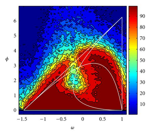
Figure 14 shows the same numerical analysis for the Rosenbrock function defined in ℝ10, both in the PSO (α = 1) and GPSO cases (Δt = 0.8 and α = 1), under the same tolerance requirements. As the number of dimensions increases, the best parameter sets seem to fit better the limit of the second-order stability. Also, the region of negative inertia values seems to be more important in size than in dimension 2. In the GPSO case, the “good” parameter region increases its size.
7.1. Time-step adapted GPSO algorithms
As a result of the above-mentioned analysis and numerical experiments, we propose the following algorithm.
- (1)
To specify the search space limits, and to initialize swarm positions randomly within, velocities are initialized to zero and are not limited.
- (2)
To choose the parameters for the standard PSO (Δt = 1), as a general rule, a good choice is an inertia value ω in the range (0.5,0.8) and a total acceleration given by (44). For cost functions with multiple local minima, inertia values in (−0.6, − 0.5) and total acceleration following the same rule (44) seem to give also very good results.
- (3)
At the exploration stage, the local acceleration ϕ2 should be bigger than the global term, ϕ1 (α < 1).
- (4)
At the convergence stage, we propose two different variants with respect to the PSO case.
(a) GPSO algorithm with Δt < 1 The idea is to monitor the percentage of models having at least one parameter on the lower or upper limit of the model search space as a function of iterations. If this percentage decreases significantly (which is expected mainly in the convergence stage), the time step Δt is reduced (e.g., Δt = 0.8 − 0.9) in order to adapt the PSO amplitudes to locate accurately the minima. Numerical experiments have shown that at the exploration stage it is common that some model parameters reach the search space limits. Nevertheless, this circumstance does not necessarily imply a time-step reduction. On the contrary, at the convergence stage it is important to adapt the PSO amplitudes in order to efficiently locate the optimum.
(b) Mixed GPSO algorithm This algorithm consists in adopting Δt = 1.2 and 0.8 alternatively for the odd and even iterations. When Δt = 1.2 the exploration capabilities increase (higher variance to avoid local minima) and for Δt = 0.8 the search is done more accurately around the global best.
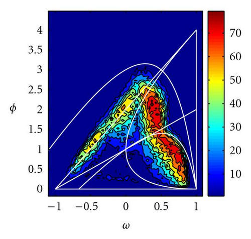
We ran several numerical experiments with the Rosenbrock, DeJong, and Griewank functions. Figure 15 shows the percentage of times (over 100 simulations) that mixed GPSO arrives very close (within a tolerance of 10−5) to the global optimum after 100 iterations. It can be observed that good parameter regions are close to both hyperbolas of the second-order stability (Δt = 1.2 and Δt = 0.8).
8. Application to an Environmental Real Case
The vertical electrical sounding (VES) is a geophysical direct current technique aiming to characterize the depth-variation of the resistivity distribution of a stratified earth. The VES methodology is as follows.
- (i)
On the surface, at each measuring station, two current electrodes and two potential electrodes are symmetrically laid at both sides of a fixed central point.
- (ii)
In successive stations, the two external current electrodes are moved apart from each other, increasing their mutual distance, while holding the two inner potential electrodes fixed in place at a much shorter distance. At each position of injection the voltage difference, ΔV, is then measured.
The inverse problem consists in estimating the conductivity and thicknesses of the stratified earth that explains the voltage measurements made on the surface. One, then, needs to define a misfit function to quantify the distance between observations and predictions issued from the earth models. This geophysical inverse problem is nonlinear and ill-posed, that is, different sets of earth models may give similar voltage predictions. In fact, the VES objective function has the minima in a very narrow and flat valley [14], similar to the Rosenbrock case in several dimensions.
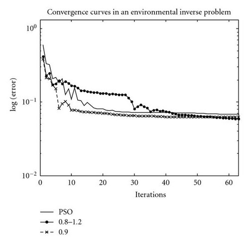
Figure 16 shows the convergence curves (logarithmic error versus iterations) for a VES geophysical inverse problem having an important environmental application (salt intrusion in a coastal aquifer), using different GPSO versions. The cost function is in this case defined in ℝ11. As it can be observed, GPSO with Δt = 0.9 performs better than PSO from the first iterations. The mixed GPSO algorithms perform more slowly, nevertheless, it is the PSO variant that reaches the lower misfit. These results obviously depend on the search space size.
9. Conclusions
A new PSO algorithm, generalized PSO, has been presented and analyzed. It comes from the continuous PSO model by considering time steps different from the unit (PSO). Its deterministic and stochastic stability regions and their respective asymptotic velocities of convergence are also a generalization of those of the PSO case. A comparison to PSO and to the continuous model is done, confirming that GPSO properties tend to the continuous as time step decreases. The size of the time steps is thus presented as a numerical constriction factor. Properties of the second-order moments—variance and covariance—serve to propose some promising parameter sets. High variance and temporal uncorrelation improve the exploration task while solving ill-posed inverse problems.
Comparisons between PSO and GPSO, by means of some numerical experiments using well-known benchmark functions and real data issued from environmental inverse problems, show that generalized PSO is more effective than PSO at accurately locating the global minimum of these cost functions. Based on this analysis, we propose two new time-step adapted PSO variants, GPSO, and mixed GPSO that improve the convergence performance of PSO in a geophysical inverse problem in ℝ11.


