A spatial model for the representation of emotional landscapes
Abstract
This article proposes a cartographic solution to represent the emotional landscapes of evasion for a Holocaust survivor, specifically his perceptions of safety or danger during his escape. The victim's emotional landscapes are spatially interpolated using techniques for vectors of both travel direction and magnitude (of perceptions of safety or danger). The implications for the spatial representation of emotions are that emotional landscapes might be better understood by going through an interpolation process, as the statistical analysis reveals spatial trends and autocorrelation. This may help in understanding how the abstract notion of space and the human valence of place vary in relation to each other (or not), and whether and how that variation differs based on distance and direction.
1 INTRODUCTION
In this article, we propose a cartographic model to represent the emotional landscape of Peter Feigl, a survivor of the Holocaust. In recent years, geographers and historians studying the spatiality of the Holocaust through the analysis of testimonies of survivors have tended to move away from traditional cartographic representations (Knowles et al., 2021) in an attempt to portray relational space and emotional place (Miranker & Giordano, 2020). While such an approach has been beneficial in exploring new ways of representing diverse social and affective data, the gap it leaves is the disconnection of the qualitative data from the locational setting, thus sacrificing potential insights into the connections between space and place. The objective of this research is to explore the feasibility of mapping qualitative data while preserving Euclidean space through an analysis of the spatially dependent emotional places of one Holocaust survivor, specifically his perception of safety or danger during his flight to safety. Are the results of the interpolation spatially and platially accurate, and is the visualization effective? Can spatial interpolation of emotion using vectors of direction and magnitude help to further develop a GIS of place? To answer these questions, we engaged in a close reading of the transcript of Feigl's recorded testimony (Feigl, 1997) and his published diary (Feigl, 2002) to estimate Feigl's emotional state during his flight to safety in southern France from June 1940 to May 1944. We then represented his emotional landscape, as we interpreted it, through spatial interpolation of both travel direction and emotion, using nonlinear interpolation techniques for vectors of direction (spatial) and magnitude (of perceptions of safety or danger). The result is an interpolated raster surface map of Feigl's journey, visualized in a vector format, across the south of France in the period from 1940 to 1944.
2 LITERATURE REVIEW
The study of the geography of the Holocaust takes place at the intersection of several disciplines, including geographic information science (GISc), geography, history, and Holocaust studies. Foundational to this research is the idea of the “spatial humanities,” that is, that GISc can contribute to informing an understanding of the humanities through spatial analysis. Historians and geographers have allied under the GIS umbrella, but as Knowles (2014) notes, many historians are uncomfortable with the quantitative focus of GIS, and gaps in theory, methodology, epistemology, and pedagogy need to be addressed. Underpinning the research presented here is the idea that geography has something substantive and original to say about the Holocaust. Around the time that historical GIS first appeared, Charlesworth (1992) issued his call for geographers to turn their attention to the Holocaust, a genocidal event that took different forms in different places. Charlesworth's plea has been answered in two ways. The first has been built against the background of historical understandings of Nazi political, economic, military, and spatial motivations, theory, and practice (Adey, 2020; Barnes, 2015; Barnes & Claudio, 2013; Clark et al., 1996; Danielsson, 2009; Egbert et al., 2016; Rössler, 1989). The second, into which this research falls, started from the spatial analytical and quantitative perspective of GISc to evolve into a mixed methods approach that attempts to move away from focusing on the perpetrator and his genocidal reorganization of space to explore narratives and testimonies of survivors. This progression can be seen, for example, in the temporal arc of Cole and Giordano's research on the Budapest ghetto, which started with mapping the shapes of the ghetto (Cole & Graham, 1995), followed by the creation of a historical GIS of the Holocaust in the city in search of meaningful spatial patterns (Cole & Giordano, 2014; Giordano & Cole, 2011), and leading to recent efforts (Giordano et al., 2022; Giordano & Cole, 2018, 2020) to develop a GIS of place incorporating narratives and testimonies (Agnew & Duncan, 1989; Tuan, 1977). These more recent works incorporate traditional GIS and mapping but analyze testimonies through methods such as corpus linguistics (CL), natural language processing (NLP), and social network analysis, and they integrate geographical concepts of space and place.
Tuan (1991) defines geography as the study of the earth (“space”) as the home (“place,” as created by humans) of people. Place, for Tuan, is stability and experience, a pause in movement where location or space is transformed into place (Tuan, 1977), or home. Agnew and Duncan (1989) build on Tuan's definitions of place by dividing place into three components, with one of them (“location”) essentially constituting space. The other two include “locale,” defined as the social setting, relationships, and structures of human experience that exist in a location, and “sense of place,” the lived and emotional experiences that create attachment, or perhaps aversion, in the human understanding of a location. Agnew and Duncan contend that all three components are necessary and complementary in the definition of place. Cresswell (2009), however, notes that place is also socially constructed, and is not so easily explained by an essentialist position (Cresswell, 2004). The French geographer, Berdoulay (1989), sees place as meaning and as grounded in social relations, with subject and landscapes interacting together to build meaning.
Some of the challenges of working with qualitative data, including testimonies, in a GIS come from uncertainty in spatial representation, which is often inherent in historical data, and challenges in the representation and analysis of narratives and testimonies. By their nature, places and spaces in survivor testimony interviews are not always easily assigned coordinates in the traditional GIS sense, as they are often vaguely defined and remembered. As concerns specifically Holocaust testimonies, ways of representing such spaces and places have been proposed by, for example, Cole and Hahmann (2019) via QSR (Qualitative Spatial Representation)—essentially a redesign of spatial databases to handle the output from natural language sources—and by Blanke et al. (2020), who used machine learning algorithms to model the components and characteristics of texts and conducted contextualized sentiment analysis on transcripts of Holocaust survivor testimonies. One obvious extension of this approach is through the use of AI, which we are experimenting with ourselves. Knowles et al. (2021) discuss using CL and NLP with Holocaust testimonies, using geoparsing to approach the texts spatially and demonstrating their use on a small sample of testimonies.
In the context of working with qualitative data in traditional GIS, especially challenging is to measure, analyze, and visualize spatially dependent emotions and experiences, although progress has been made (Hauthal & Burghardt, 2016; Hawthorne et al., 2022), including attempts at automated methods of measuring emotion spatially (Huang et al., 2020; Shoval et al., 2018). These efforts have been primarily concerned with present-day data, (Pánek, 2018; Zeile et al., 2015) and the use of historical data is more rare, but see Pearce (2008). Recent cartographic research has looked at the relationship between colors and visualized emotions and at how viewers perceive congruity (or not) in the cartographic rendering of those emotions (Kushkin et al., 2024). Research on spatial interpolation of qualitative data—the method chosen for our project—has also been ongoing, mostly in the context of geolinguistics (Chagnaud et al., 2017; Hoch & Hayes, 2010; Lowry, 2022), but see also Musafer et al. (2017) work on spatial modeling when multiple variables have a nonlinear spatial dependence. In visualization, both theory and case studies support the notion that users' enthusiasm to interact with the visualization increases as actual data are included (Lloyd & Dykes, 2011), hence our attempt at mapping lived experiences and emotions in the spaces and places where they occurred.
3 PETER FEIGL'S STORY
Peter Feigl was born to a non-religious, relatively well-off Jewish family in a suburb of Berlin, Germany in 1929. From Berlin, the family moved first to Prague, then to Vienna, and finally to Brussels only days after Germany annexed Austria in March 1938. When Germany invaded Belgium in May 1940, Peter, his mother, and his grandmother (his father had been arrested) fled to France, where Feigl spent the next 4 years until his escape into Switzerland in May 1944. During the stay in France, his father was reunited with Feigl and his mother, but his parents were captured in August 1942, and unbeknownst to Feigl, deported to Auschwitz, where they were likely murdered on arrival. Feigl spent nearly 2 years in France with other caregivers and protectors until his flight to safety (Feigl, 1997, 2002).
The temporal and spatial focus of this research is the period from June 1940 to May 1944, when Peter was in southern France. During this time, the governing powers in this area were first the Nazi collaborationist Vichy regime, which came to ascendancy after France's surrender to Germany in June 1940, then in November 1942, the Germans moved their forces into southern France and took direct control (Marrus & Paxton, 2019; White, 2019). Our region of interest is roughly 250 by 500 km, starting from Bordeaux on the Atlantic Ocean, where Feigl is at the beginning of the study period, to Camp de Gurs, a concentration camp directly south of Bordeaux closer to the Spanish border and in the foothills of the Pyrenees Mountains, to the Marseilles area on the Mediterranean, to Geneva, Switzerland, where Feigl escapes to safety at the end of the study period. Most of the four-year period was spent in several small towns and villages in the middle of this bounded area, with over 2 years in total in Auch with his mother and then with both his parents and about two-thirds of a year each in Le Chambon-sur-Lignon and Figeac. These smaller communities tended to be remote and isolated. Le Chambon-sur-Lignon was a significant place for rescue and harboring of Jewish refugees during the Holocaust, on which much has been written (Bolle, 1992; Browning, 2016; Henry, 2016; Moorehead, 2014; Rochat & Modigliani, 1995; White, 2019).
A child as the Holocaust began, Peter kept a diary which documented his experiences (Feigl, 2002) and was also interviewed as part of USC Shoah Foundation's Visual History Archive (VHA) (Feigl, 1997). Written for his parents, the diary begins on August 27, 1942, when he learns of their arrest, and continues until February 1, 1943, when it was likely paused due to concerns by Feigl's caregivers in Le Chambon-sur-Lignon about what would happen if the diary was found. The diary picks up again on January 1, 1944, with Feigl at school in a different location, Figeac, and it continues until he gets to Switzerland in May 1944, describing his flight to safety from Figeac through Clermont-Ferrand, Lyon, Viry, and into Switzerland, with a few additional entries in June 1944 (Feigl, 2002). On April 18, 1997, Feigl was interviewed for the VHA at his home in Palm City, Florida. The 2-h video interview recorded Feigl's memories of his life before, during, and after the Holocaust. A transcript of the interview was obtained for this research from the USC Shoah Foundation (Feigl, 1997).
4 THE CODING PROCESS
Our analysis started with the coding of Feigl's life experiences, which were categorized according to their temporal, spatial, and social elements, and organized in an Excel table (partially reproduced in Table 1), with columns for “date,” “location,” “event,” “person,” “foe or friend rating,” “source,” and “other locations mentioned.” Human-coding is subjective (Blanke et al., 2020) and is acknowledged as a source of possible bias and error.
| Date | Location | Event | Person | FoeFriendRating | Source | Other locations mentioned |
|---|---|---|---|---|---|---|
| 05-06-1940 | x | Mother went to French police, then gendarmerie, then prefecture, to get permission to live in Bordeaux | MTH | 10 | t | |
| 05-06-1940 | x | Mother went to French police, then gendarmerie, then prefecture, to get permission to live in Bordeaux | POL | 5 | t | |
| 05-06-1940 | x | Mother went to French police, then gendarmerie, then prefecture, to get permission to live in Bordeaux | GDX | 5 | t | |
| 05-06-1940 | x | Mother went to French police, then gendarmerie, then prefecture, to get permission to live in Bordeaux | PRE | 3 | t | |
| 05-06-1940 | x | Prefecture tells the mother to take a train to Oloron-Sainte-Marie. They know what to do with cases like yours | PRE | 3 | t | Oloron-Sainte-Marie |
| 05-06-1940 | x | Prefecture tells the mother to take a train to Oloron-Sainte-Marie. They know what to do with cases like yours | MTH | 10 | t | Pyrenees |
| 06-06-1940 | n | Mother buys a train ticket to Oloron-Sainte-Marie for her, PF, and grandmother | MTH | 10 | t | |
| 06-06-1940 | n | Mother buys a train ticket to Oloron-Sainte-Marie for her, PF, and grandmother | GMH | 9 | t | |
| 06-06-1940 | n | Arrive at train station, surrounded by gendarmerie with submachine guns. Took off train, loaded onto truck | GDN | 2 | t | |
| 06-06-1940 | u | They were taken to Camp de Gurs, infamous French internment camp built for Spanish communists | GDN | 2 | t | |
| 07-06-1940 | u | In camp with thousands of other refugees. Horrible conditions, very little food | REF | 6 | t | |
| 07-06-1940 | u | Mother selected as barracks chief. PF in same barracks as mother and grandmother | MTH | 10 | t | |
| 07-06-1940 | u | Mother selected as barracks chief. PF in same barracks as mother and grandmother | GMH | 9 | t | |
| 08-06-1940 | u | Mother went everyday to nuns running food distribution, borrowed little extra food | NUN | 6 | t | |
| 15-06-1940 | u | Mother had argument with one nun about such little food. Nun insulted refugees, mother slapped her | MTH | 10 | t | |
| 15-06-1940 | u | Mother had argument with one nun about such little food. Nun insulted refugees, mother slapped her | NUN | 3 | t | |
| 15-06-1940 | u | Mother was begging food for people who were starving, including elderly, some of whom were dying | MTH | 10 | t | |
| 15-06-1940 | u | Mother was begging food for people who were starving, including elderly, some of whom were dying | REF | 6 | t | |
| 01-07-1940 | u | France surrendered, Germans coming to inspect the camp | GER | 1 | t | |
| 01-07-1940 | u | Mother pushed herself to the German delegation, showed her German passport, demanded the release | MTH | 10 | t | |
| 01-07-1940 | u | Mother pushed herself to the German delegation, showed her German passport, demanded the release | GMH | 9 | t | |
| 01-07-1940 | u | Mother pushed herself to the German delegation, showed her German passport, demanded the release | GER | 1 | t | |
| 01-07-1940 | u | German commander taken aback, ordered her release, and for a cab to take her anywhere | GER | 1 | t | |
| 01-07-1940 | u | Cab driver arrives within 30 min, asks where to go, mother says “north” since the Spanish border closed | CAB | 5 | t | Spain |
| 01-07-1940 | h | They arrived Auch, but could not go any further due to German troops ahead, said refugees heading toward them | CAB | 5 | t | |
| 01-07-1940 | h | They arrived Auch, but could not go any further due to German troops ahead, said refugees heading toward them | REF | 6 | t | |
| 01-07-1940 | h | They arrived Auch, but could not go any further due to German troops ahead, said refugees heading toward them | GER | 1 | t |
“Date” corresponds to either the exact date referenced in the diary or testimony; when no exact date was given, an estimate was made based on known historical facts or personal events in Feigl's life. In case of disagreement between the diary and the testimony, diary dates were used as the diary was written in the immediacy of the events in question, rather than recollected decades later. Some rows contain multiple entries for the same date, which will be explained when discussing the “person” column. Note that the estimated dates have a degree of uncertainty, but this uncertainty was not recorded nor visualized as it was usually a matter of a few days and therefore did not significantly affect the results of the analysis for the period of study. “Location” refers to the city, village, or (rarely) a specific address in which the events occurred as recorded in the sources. Each location was assigned an alphabetic code (e.g., Bordeaux is an “x”) to facilitate later analysis. The column “event” contained a summary of what the diary or testimony discussed; this column was added to facilitate close reading and was not used in the analysis or for the visualization. “Person” records every reference in the diary or testimony to people Feigl had immediate contact with, including a few instances found in written letters. “Person” can refer to an individual (e.g., mother) or a group of individuals (e.g., German soldiers), and each person was given a three-letter code. When multiple persons are discussed in the same diary or testimony entry, multiple rows for the same date are used to record every person referenced separately in their own row. The “person” column represents the social network of Feigl, including brief contacts. Note that 16 of the 309 “person” rows have no specific individual(s) recorded. In most cases, this occurred when Feigl was writing or speaking about locations he was not at but simply referred to (column “other locations mentioned”). There was also one entry without a “person” in reference to a friend's parents whom he did not meet but who his guardian at the time helped, and three entries where no “persons” were mentioned (in Clermont-Ferrand and Lyon). These three were nonetheless included in the analysis because of their relevance to Feigl's narrative. The foefriendrating column is a numerical estimate on a 1–10 scale, based on Feigl's characterization of whether that person represented a “foe” or a “friend.” The lowest values are for foes (representing “danger”), the middle ones are neutral, and the highest values are for friends (representing “safety”). A rating of “10” was reserved for Feigl's parents; “9” was generally used for other family members or direct caregivers and protectors; “8” was other aid organizations such as the Quakers, teachers, and close school friends; “6” or “7” were other students and refugees; “5” were students he did not get along with or bystanders, such as a cab driver; “2,” “3,” or “4” were generally Vichy French administration officials or gendarmes who posed varying levels of risk to Feigl; and “1” were German military or officials, gendarmes sent to arrest Feigl, or police searching for escapees at the border with Switzerland. These categorizations are subjective and based on interpretations of Feigl's perceptions as reported in his diary and testimony. As an example, in March 1938, Feigl writes about going to a square in Vienna, seeing the large crowds and the Hitler youth, and listening to Hitler's speech. As he writes, “I was caught … in the spirit of this … I wished I could join them” (Feigl, 1997). He then went home and excitedly told his mother about seeing “our führer.” His mother quickly disabused him of such a positive assessment, and in fact within days the family had left Vienna for Brussels. Nonetheless, we gave this event a rating of “8” on the foefriendrating scale, because at the time the event was perceived in positive terms, and Feigl did not feel threatened. Finally, “source” records whether the data in the row was from the diary or the testimony, and “other locations mentioned” recorded Feigl's references to places he was not at the time. These two columns are for reference only and were not used in the analysis.
Overall, the table includes 309 entries covering the period 1929–1944, which were organized by date and then by location, with foefriendrating values averaged for each. Latitude and longitude coordinates (Pridal et al., 2019) were assigned to each date and location (see Table 2 below for a partial view) and then entered in ESRI's ArcGIS Pro, where the entire analysis was performed.
| Date | Location | AvgFriendFoeRating | Longitude | Latitude |
|---|---|---|---|---|
| 05-06-1940 | x | 6.0 | −0.58619 | 44.86351 |
| 06-06-1940 | n | 7.0 | −0.59541 | 43.16789 |
| 06-06-1940 | u | 2.0 | −0.75907 | 43.27716 |
| 07-06-1940 | u | 8.3 | −0.75907 | 43.27716 |
| 08-06-1940 | u | 6.0 | −0.75907 | 43.27716 |
| 15-06-1940 | u | 7.3 | −0.75907 | 43.27716 |
| 01-07-1940 | u | 4.5 | −0.75907 | 43.27716 |
| 01-07-1940 | h | 6.5 | 0.566575 | 43.66248 |
5 METHODS
The Mean Average-Friend-Foe-Rating value was calculated based on the ratings in Table 2 and as the average for all dates at that location. This gives an overall rating of whether that location was “safe” (where Feigl was more often in contact with friends) or “dangerous” (where Feigl was more often in contact with foes). Since our study only covers the period June 1940–May 1944 (Bordeaux to Geneva), the dates and locations prior to Bordeaux in June 1940 were discarded; this left us with 19 locations, three of which (Auch, Condom, and Les Caillols) had two entries due to separate and noncontiguous time periods spent there.
- Convert degrees to radians and calculate vector for U (or X)
- Convert degrees to radians and calculate the vector for V (or Y)
A parallel can be made between how we mapped Feigl's journeys across southern France and how wind is represented cartographically as a vector with two components: a direction and a magnitude (or speed). In our analysis, “magnitude” is measured by the foefriendrating value for the locations Feigl visited between Bordeaux and Geneva from 1940 and 1944. The foefriendrating value is considered to be an indicator of Feigl's emotional state, with the range of perceptions from danger to safety corresponding to emotions from fear to calm (Russell, 1980; Sandler, 1960). “Feeling safe” is a prerequisite to most positive emotions (Fredrickson, 2000), and from a geographical perspective, the idea of Geborgenheit more precisely correlates safety with being nested within a sheltering place, having a positive sense of well-being, and a relative lack of fear (Hutta, 2009), all of which are partially a result of one's social contacts. In the magnitude and direction of the foefriendrating, therefore, we are representing Feigl's emotional pathways in space and time, based on the metaphor that even as wind flows, moves, and varies in magnitude and direction across the landscape, so too did Feigl's experiences of danger and safety flow, move, and vary in magnitude and direction as he journeyed for survival. The magnitude and direction of Feigl's emotions related to danger and safety are both necessary to interpolate with the research goal specifically to test methods for representations and understandings of spatially dependent emotions. Spatial interpolation has been proposed as a way to visualize non-geographic information (Skupin & Fabrikant, 2003), such as the emotional data in this research.
Spatial interpolation is defined as the estimation of attribute values at locations without a known measurement based on locations where the value is known. Bolstad and Manson (2022) make a distinction between spatial interpolation and spatial prediction. The former is based on a predefined algorithm and estimated parameters and constants, and its value can be exact, in the sense that interpolated points may be equal to known values at those measured locations. Examples of spatial interpolation methods include nearest neighbor and inverse distance weighted (IDW). Spatial prediction is based on applied statistical fitting of the model to the spatial and non-spatial data, often with independent variables, and can directly address spatial autocorrelation and cross-correlation. Examples of spatial prediction methods include trend surface and several forms of kriging. Here we use the term spatial interpolation in the broader sense, inclusive of Bolstad and Manson's definitions of both spatial interpolation and spatial prediction methods.
The choice of an appropriate spatial interpolation method is based on the nature of the data and prediction being made. Here we use ordinary kriging. Other techniques were considered but rejected, including the nearest neighbor, fixed radius, IDW, spline, and trend surface-simple spatial regression methods. Compared with these, ordinary kriging retains three desirable characteristics: (a) it measures spatial trends (the value of the variable changes based on direction); (b) it describes the local spatial autocorrelation, measured similar to Geary's C, and then uses the distance-based change in spatial autocorrelation (using the concepts of lag distance and semi-variance, plotted on a semi-variogram) to estimate values at unknown locations; and, (c) there is a stochastic (nonlinear, random) variation. Like IDW, ordinary kriging uses weights, but here the weights are chosen based on statistical optimization using the semi-variogram. The determination of “optimal” weights is based on minimizing errors and variance in the predictions (Bolstad & Manson, 2022). Note that in a previous study mapping emotions, IDW was chosen and kriging rejected due to a lack of consensus on choosing the appropriate model of the kriging semi-variogram for emotion (Hawthorne et al., 2022). The way we overcame this problem is by exploring kriging's many different semi-variogram models and settling on a model that minimizes prediction error, and by then comparing the resulting visualizations with a close reading of Feigl's narratives. We also considered other versions of kriging (O'Sullivan & Unwin, 2010), ultimately discarding them all as inappropriate to the subject data due to their assumptions about means and/or multiple variables.
Spatial interpolation using ordinary kriging was performed over three iterations on the two directional vectors (U and V) and on the magnitude data itself (the mean values for foefriendrating for each time period at a location). The most crucial step in the analysis consisted in choosing the appropriate semi-variogram model and the related parameters, which we did through a process of cross-validation (Gundogdu & Guney, 2007; Pasini et al., 2014). To determine the best fit for the data and the most appropriate model, we went through several different iterations testing the model options available within ArcGIS Pro. For each iteration, the measured errors (mean, RMSE, mean standardized, RMSE standardized, and average standard error) were recorded in a table. To reduce the number of iterations and keep the task to a manageable size, one of the models was kept constant and then different parameter choices within that method were run, looking for the lowest values for RMSE and the other error measures; those parameter settings were then used in each of the other models. We acknowledge that this does not guarantee the best choice, but it is the most efficient given our analytical objectives. Also, for each model, ArcGIS Pro offers an “Optimize” option, which was chosen every time. The option configures the ideal lag size, number of lags, nugget, range, and sill in order to minimize error. Tables 3 and 4 are examples of the cross-validation data used (with Table 4 the continuation of Table 3) to choose the model for interpolating the magnitude of the mean foe-friend measure.
| Mean friend/foe | ||||||||||
|---|---|---|---|---|---|---|---|---|---|---|
| Method | Ordinary kriging | |||||||||
| Type | Prediction | |||||||||
| Transformation/Trend removal | No | |||||||||
| Optimized | Yes | |||||||||
| Number of lags | 12 | |||||||||
| Model | J-Bessel | Sphere | Circular | TetraSph | PentaSph | |||||
| Anisotropy | FALSE | TRUE | FALSE | TRUE | FALSE | TRUE | FALSE | TRUE | FALSE | TRUE |
| Neighborhood type | Standard | |||||||||
| Max/Min Neigh | 5, 2 | |||||||||
| Sector type | 4 with 45% | 8 | 8 | 8 | 8 | 8 | ||||
| Copy from variogram | TRUE | |||||||||
| Count | 16 | 16 | 16 | 16 | 16 | 16 | 16 | 16 | 16 | 16 |
| Mean | 0.18158257 | 0.182752964 | 0.004035754 | −0.070550335 | 0.019029388 | 0.012140533 | 0.013881585 | −0.04948364 | −0.05471776 | −0.08727143 |
| Root-mean-square | 1.824946708 | 2.011855219 | 1.978978273 | 2.056617294 | 1.957121503 | 2.01858213 | 1.97434846 | 2.040123113 | 1.966415738 | 2.045118991 |
| Mean standardized | 0.045122191 | 0.050205456 | −0.00120141 | −0.04165848 | 0.00021786 | −0.0059004 | 0.002028194 | −0.0346578 | −0.032299598 | −0.05320096 |
| Root-mean-square standardized | 1.172406631 | 1.283255641 | 1.014309738 | 1.032434904 | 1.021323747 | 1.025065356 | 1.020153227 | 1.025936187 | 1.020734291 | 1.033001126 |
| Average standard error | 1.824640795 | 1.667866996 | 1.948250107 | 1.985876608 | 1.89316135 | 1.930541754 | 1.926932488 | 1.970665789 | 1.920972909 | 1.965374543 |
| Mean friend/foe | ||||||||||||
|---|---|---|---|---|---|---|---|---|---|---|---|---|
| Method | Ordinary kriging | |||||||||||
| Type | prediction | |||||||||||
| Transformation/Trend removal | No | |||||||||||
| Optimized | Yes | |||||||||||
| Number of lags | 12 | |||||||||||
| Model | Exponential | Gaussian | Rational Quad | Hole Effect | K-Bessel | Stable | ||||||
| Anisotropy | FALSE | TRUE | FALSE | TRUE | FALSE | TRUE | FALSE | TRUE | FALSE | TRUE | FALSE | TRUE |
| Neighborhood type | ||||||||||||
| Max/Min Neigh | ||||||||||||
| Sector type | 8 | 8 | 8 | 8 | 8 | 8 | ||||||
| Copy from variogram | ||||||||||||
| Count | 16 | 16 | 16 | 16 | 16 | 16 | 16 | 16 | 16 | 16 | 16 | 16 |
| Mean | 0.074268083 | 0.061627895 | 0.042824784 | 0.03386517 | 0.076453455 | 0.051163672 | 0.09251155 | 0.116725804 | 0.078717905 | 0.046566061 | 0.082266143 | 0.045507224 |
| Root-mean-square | 2.015840847 | 2.080235794 | 1.998201605 | 2.056813198 | 2.01540973 | 2.08639963 | 1.945652488 | 2.052528425 | 2.009916113 | 2.050885731 | 2.01106623 | 2.052355537 |
| Mean standardized | 0.022703162 | 0.008215225 | 0.012093584 | 0.002577731 | 0.02285441 | 0.000494145 | 0.025735614 | 0.0250635 | 0.024986323 | 0.002816245 | 0.026676021 | 0.002753946 |
| Root-mean-square standardized | 1.064119463 | 1.120022273 | 1.024230341 | 1.073420645 | 1.06135627 | 1.116872904 | 1.136011555 | 1.192906451 | 1.05784205 | 1.101812293 | 1.055478021 | 1.097538907 |
| Average standard error | 1.848436795 | 1.790384453 | 1.916860907 | 1.883434915 | 1.860971019 | 1.808342851 | 1.673371754 | 1.661482043 | 1.856637445 | 1.796202023 | 1.866850737 | 1.806388126 |
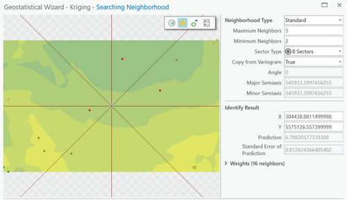
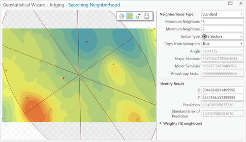
The next step in choosing a semi-variogram model consists of determining how well the derived raster surface portrays the known and interpolated data, including their spatial variability. For the mean foefriendrating, the Rational Quadratic method with anisotropy, which considers direction as well as distance (see bolded column in Table 4), had both low values for error and the most accurate raster surface. Figures 1 and 2 give an example of how the raster surfaces were compared for the different models: Figure 1 shows the results using the spherical model, which results in smooth surfaces without much detail, while Figure 2 shows the surface resulting from the rational quadratic model, which more closely preserves the inherent variability of Feigl's emotional states. In both cases, the edge effect is prominent, with loss of detail in Bordeaux (middle left), Camp de Gurs (lower left), multiple points around Marseille (lower right), and three points around Geneva (upper right). This was true of all semi-variogram models tested.
- Quadratic variogram model (OpenGeomatics, 2023)
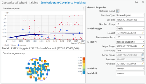
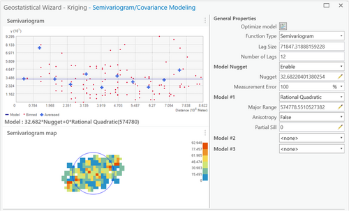
As can be seen in Figure 3, the mean friend-foe data was S-shaped (see “+'s” for the averaged data in the lags). The model does not appear to strictly follow the “S,” especially in this running with the anisotropy set as “true,” but nonetheless, it does capture the spatial pattern in the semi-variogram.
- Combine vectors for U and V and convert radians to degrees
The final step in the procedure consisted in merging the combined results of the interpolated directions with the interpolated raster of the magnitude of mean foefriendrating. The visualization of the resulting raster was accomplished as a vector field, with band 1 being magnitude (mean foefriendrating) and band 2 being direction (now converted to angle degrees).
To test the robustness of the results, two additional iterations of the complete process, from interpolation forward, were performed. In both, we kept the interpolation of the magnitude of mean foefriendrating from the first iteration, which we considered satisfactory. What changed was how the directional vectors were interpolated, which in our estimation was not accurate. In both iteration two and three, for the interpolation of the directional vectors (U and V) and when two or more samples are at the same location, for those coincident points, the author chose to “Include All” samples. Additionally, in iteration three, for the semi-variogram model, the maximum and minimum neighbors were both changed to one and the sector type to eight. Given these parameters, iteration three provided the most accurate interpolation.
Figure 4 shows the steps followed in the analysis.

6 DISCUSSION OF RESULTS AND FINDINGS
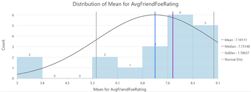
In this article, we attempt an interpretation of Feigl's experience and emotional status through his writings and video interview, read through the lens of his social contacts and impressions at each location. Crucially, the two sources we use are diversified, both chronologically and as concerns the recording media. For Feigl, as expected, there were places of safety (Auch, for example, where he lived with his parents for over 2 years) and places of danger (Clermont-Ferrand). As we are dealing with human behavior, the statistical distribution of the mean foefriendrating value in Figure 5 is not a classic Gaussian distribution, but patterns do emerge.
The semi-variogram model for the interpolation of magnitude of mean foefriendrating, as shown in Figure 3, shows that at the closest distances and then again at the middle distances, there is relatively high spatial autocorrelation; in between those close and middle distances, and then again at larger distances, there is much higher semi-variance. Given that the study area is approximately 250 × 500 km, what this means is that the emotional data is spread out, with a long range before the sill is reached, with high spatial autocorrelation at short distances, but then less of a spatial trend after that. By using the rational quadratic model, the ordinary kriging method can capture this trend, and effectively interpolate it, and therefore, the method is deemed appropriate based on consistency with the assumptions outlined above.
For the mean foefriendrating interpolation, as seen in Table 4, error statistics are summarized in Table 5. The rational quadratic model did not always perform the best, but overall had strong results in all measures, with mean error and mean standardized error both close to zero; the rational quadratic model had the lowest mean standardized error of any models, very close to zero. The RMSE and the average standard error should also be relatively small. None of the models have ideal RMSE or average standard errors, but the root-mean-square standardized error (RMSSE), which should be close to one, reflects good accuracy statistics (Gundogdu & Guney, 2007; Pasini et al., 2014).
| Count | 16 |
| Mean | 0.0511636722659467 |
| Root-mean-square | 2.08639962983321 |
| Mean standardized | 0.000494145177060777 |
| Root-mean-square standardized | 1.11687290429922 |
| Average standard error | 1.80834285072213 |
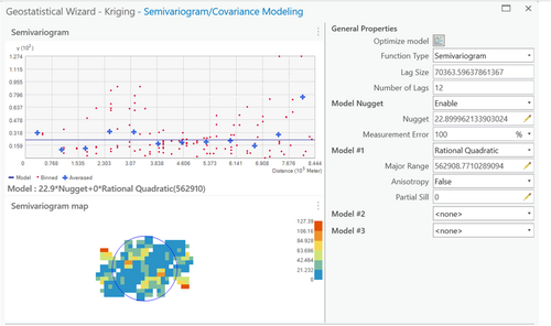
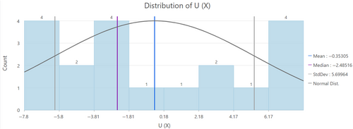
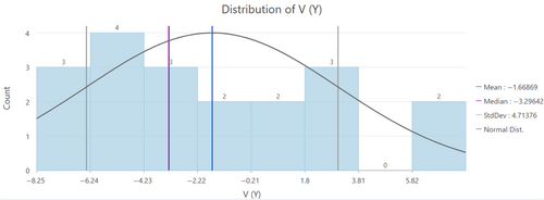
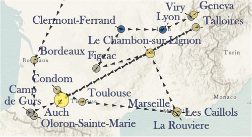
For the directional vector interpolations, there was very little spatial autocorrelation and very little spatial trend in the data, as Figures 6 and 7 show. There is also not a pronounced stochastic variation in the directional data, as can be seen in Figures 8 and 9. Both U and V have very high standard deviations. The semi-variograms for direction, as well as the distribution of data, explain why three iterations were needed to visualize direction more correctly. Since there is basically no spatial trend or autocorrelation, the inclusion of multiple points in the neighborhood definition of the model effectively dilutes the data and leaves us with an overall direction value devoid of detail, as indeed were the results in iterations one and two. Limiting the neighborhood to one sample in the third iteration forced the model to look at each instance individually and interpolate points around it only from that point. The error statistics for the interpolation of the directional vectors are presented in Tables 6 and 7, in this case for iteration 3 only. Of note, the count is 19 for the directional data because in both iterations 2 and 3, we chose to include all data when there were coincident points. While the RMSE and average standard error are relatively high, as is to be expected given the distribution of data, the other statistics are more satisfactory, particularly the RMSSE, which is very close to a value of one in both cases. From a statistical standpoint, then, the interpolated results appear acceptable given the source data. This leads, then, into a qualitative assessment of the interpolated surfaces and visualizations for each iteration based on their comparison to a base visualization of the known data points only, as seen in Figure 10 (which shows Feigl's known locations and the foefriendrating value at each location, with the size of the circles representing the length of time Feigl spent at each location). The interpolated surfaces were also assessed as concerns how well they showed directional variability in Feigl's movement in comparison to the raw visualizations in Figure 11.
| Count | 19 |
| Mean | −0.302195129662223 |
| Root-mean-square | 6.60650993250574 |
| Mean standardized | −0.0368792166946189 |
| Root-mean-square standardized | 1.03771248114911 |
| Average standard error | 6.33756330279727 |
| Count | 19 |
| Mean | 0.406866118025807 |
| Root-mean-square | 5.24307640349186 |
| Mean standardized | 0.0724878449104316 |
| Root-mean-square standardized | 0.989686460004018 |
| Average standard error | 5.30498333658098 |
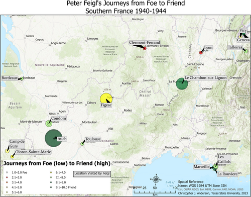
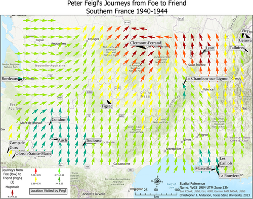
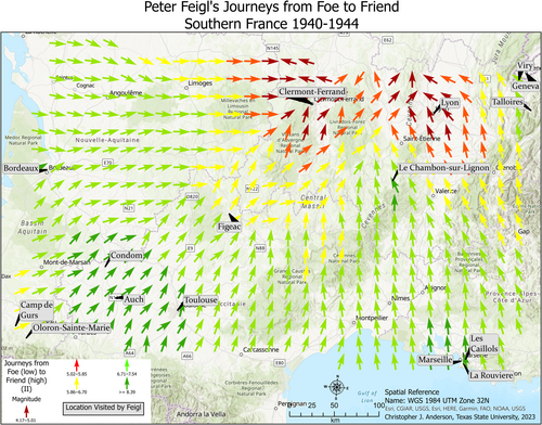
The interpolation results for iteration 1 and 2 are shown in Figures 12 and 13, respectively, based on their parameters as explained in the previous sections. Both iterations accurately reflect the magnitude of the mean foefriendrating value at each location and in the surrounding areas, but the travel vectors are overly smoothed, with an inherent loss of data, due to the lack of spatial trend and autocorrelation in the directional data as explained above. The interpolation results for iteration 3 are presented in Figure 14. As a result of limiting the neighborhood for the directional interpolation to one location only, the directional component is now much more dynamic and accurate, reflecting the multidirectional reality of Feigl's travels. There is still some smoothing of data, including at the lowest and highest ends of the magnitude of mean foefriendrating as well as in direction, and there is also an edge effect as mentioned earlier. Overall, iteration 3 offers the most effective visualization of Feigl's varying emotional landscapes across southern France from 1940 to 1944. The visualization is not intended to be a linear or even temporal map of his travels, but rather an attempt at mapping his path across the landscape as his perceptions of danger and safety varied. Importantly, it must be noted that Feigl did not have agency in his choice of travel. At first, he went with his parents, who were being directed by both authorities and events, or he went where his parents told him to go (summer camp). After his parents' arrests, Feigl was taken in by various aid organizations to save his life, moving from place to place for shelter and schooling and eventually to freedom in Switzerland. It truly was a whirlwind experience for young Peter, who was caught up in the vortex of the Holocaust, as Figure 14 visualizes well. Unfortunately for his parents, that vortex took them ultimately to Auschwitz and death.
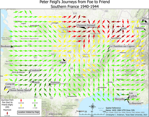
This research attempts to reflect Feigl's journeys across southern France as a moving and dynamic emotional landscape. The overall methodology was derived from how wind is interpolated, as a vector with magnitude and direction, and serves as a metaphor for how Feigl was moved across and around the landscape, all the while experiencing danger and safety. It is a novel conceptualization, and its effectiveness can be measured through the accuracy of space and place that it portrays, and in both, it appears to succeed.
7 CONCLUSIONS
The objective of this research is to explore the feasibility of applying a cartographic perspective to qualitative data, thus preserving the representation of Euclidean space, through interpolating the spatially dependent emotional places of one Holocaust survivor, specifically his perception of safety or danger during his flight to safety. The article addresses the gap in GISc of how to represent both space and place in a traditional GIS. The results of the interpolation appear spatially accurate, and the visualization effectively portrays both.
More broadly, we demonstrate how emotional landscapes might be better understood by running them through a spatial interpolation process to reveal spatial trends and the presence of spatial autocorrelation. This may help in understanding how the abstract notion of space and the human valence of place vary in relation to each other (or not), and whether and how that variation differs based on distance and direction. The resulting visualization then can reveal patterns in the landscape that are not immediately apparent through a simple linear progression, and by contextualizing the analysis and the visualization in the actual physical space, the spatial relationships that are there are preserved, honoring the victim's experiences in those places.
This research is challenged in both method and data. It is limited by the subjective coding of the survivor's testimony. Its accuracy in the portrayal of an individual's experiences is biased by the authors' interpretive frameworks, backgrounds, and knowledge. The relatively low number of data points also colors the interpolation results, particularly for a spatial extent as large as the one studied here, as do issues related to the lack of “pure” statistical conditions that would make it ideal for a fitting interpolation process such as kriging.
The opportunities provided through future extensions of this research include incorporating the temporal scale into the interpolation and visualization process. For Feigl, there were a few places in which he spent most of the time, while others were just a day or a few weeks. It would be perhaps useful to include time into the prediction model, with the ultimate goal of better reflecting the experiences of this Holocaust survivor. Automation of the emotional coding process, either through artificial intelligence or existing natural language processing tools, could allow the scaling up of this research.
CONFLICT OF INTEREST STATEMENT
There are no conflicts of interest of which we are aware.
Open Research
DATA AVAILABILITY STATEMENT
The data that support the findings of this study are available from the corresponding author upon request.


