
Bayesian Hierarchical Structure for Quantifying Population Variability to Inform Probabilistic Health Risk Assessments
Abstract
Human variability is a very important factor considered in human health risk assessment for protecting sensitive populations from chemical exposure. Traditionally, to account for this variability, an interhuman uncertainty factor is applied to lower the exposure limit. However, using a fixed uncertainty factor rather than probabilistically accounting for human variability can hardly support probabilistic risk assessment advocated by a number of researchers; new methods are needed to probabilistically quantify human population variability. We propose a Bayesian hierarchical model to quantify variability among different populations. This approach jointly characterizes the distribution of risk at background exposure and the sensitivity of response to exposure, which are commonly represented by model parameters. We demonstrate, through both an application to real data and a simulation study, that using the proposed hierarchical structure adequately characterizes variability across different populations.
1. INTRODUCTION
To quantify health risk from chemical exposure faced by sensitive populations, human variability is an important factor to consider in human health risk assessment. Traditionally, to account for this variability, an interhuman uncertainty factor (up to 10) is applied to the 100(1 − α)% lower bound of the benchmark dose (BMD). The BMD is the dose that produces a predetermined change in response of an adverse effect compared to background, and is used as a point of departure in risk assessment when estimating an oral reference dose (RfD) or inhalation reference concentration (RfC). A number of researchers have attempted to develop general quantitative methods or conceptual models to describe noncancer risk probabilistically.1-5 As agencies such as the U.S. Environmental Protection Agency (US EPA) move toward probabilistic risk assessment,6-8 new methods are needed to probabilistically quantify human variability.
We propose a Bayesian hierarchical model to quantify human variability. This is accomplished by jointly characterizing the distribution of risk at background exposure as well as the sensitivity of response to exposure using exposure-response data obtained from various populations (i.e., cohorts). Here, we define “population” as a cohort of individuals with different characteristics (e.g., gender, age, exposure, etc.) in a particular study. As this represents a cohort of individuals, such populations typically have less variability than the “target population” of interest (e.g., the entire U.S. population). In modeling the target population, the overall heterogeneity can be seen as originating from multiple sources: first, there is heterogeneity between individuals within each population, we call this interindividual variability; next, there is heterogeneity between studies, this is called interpopulation variability; and on top of that, there is variability across different populations, which is defined as interhuman (or human) variability describing the variability in the target population.
For the model, we assume that human variability in response to chemical exposure, especially in the low exposure range, is primarily affected by two factors: (1) individuals exposed at background exposure levels have different background risks, and (2) differences in genetics (e.g., resulting in different “detoxifying” metabolic rates), life style (e.g., co-exposures such as smoking that can exacerbate an individual's response to a given chemical exposure), and other factors cause individuals to have different levels of sensitivity to the same exposure level, which affect individual risks. These causes of variability will also appear at interpopulation and interhuman levels. When we only have data at the population level (like most data reported in epidemiological studies), quantifying the interpopulation variability is an important first step to a full interhuman variability quantification.
To incorporate the interpopulation variability, we construct a Bayesian hierarchical model among different subpopulations for the parameters that represent background risk and response sensitivity. Most parametric exposure-response models for continuous data contain two to four parameters with different and varying biological relevance. For example, the simplest linear model has two parameters, intercept and slope, which well correspond to these two factors. However, the Power model and Hill model with more parameters also include equivalent parameters for the two factors. In this study, we demonstrate, through both an application to real data and a simulation study, that using Bayesian hierarchical structure on partial model parameters can quantify the distribution of the background risk and response sensitivity (represented by corresponding parameters) in various exposure-response models, and it is an adequate approach to quantify variability across different populations.
The article is organized as follows: in Section 2., the fundamental methodology is outlined. Section 3. presents the results from an analysis of a set of studies using the proposed method. A simulation study is described in Section 4.. Finally, Section 5. offers a comprehensive discussion.
2. METHODOLOGY
We propose a Bayesian hierarchical model to quantify the variability and uncertainty in human populations with a focus on the low-exposure region. In particular, we fit an exposure-response model to data sets from different studies, where the subjects in the studies have the same or extremely similar endpoints and exposure metrics, and comparable external conditions, geographically, economically, etc., and build hierarchical structure over the parameters of interest (i.e., background risk and response sensitivity) to characterize their distributions across different populations. In the hierarchy, the higher-level distribution is used to estimate the distribution of relative risk at any given exposure level. The higher-level distributions describing the interpopulation heterogeneity will lead to heavier tailed distributions of relative risk, which will appropriately quantify the variability across populations and better estimate the interhuman variability.
2.1. Exposure-Response Modeling
 (1)
(1) represents the mean at exposure
  ;
;  is the expected value of cases adjusted for demographics (e.g., person-years, age, sex, etc.); and
  is an exposure-response function with a vector of parameters β representing relative risk due to exposure to a chemical of interest.
The cohorts used in this study all have an internal referent (i.e., the group with the lowest exposure d1), and the expected values are themselves estimated from the same data as the model parameters. To account for this in the model, we define  (where
  is a common exposure-response function). This adjusts the models by dividing out the exposure contribution at reference group d1. This forces the fitted relative risk at the reference group to be 1. In addition, because the denominator is a constant given estimated model parameters,
  has the same mathematical format as the
  .
.
 (the expected values reported in or derived from summary data in published literature) and o1 is equal to the ratio of ei and e1, that is:
 (2)
(2) . Therefore, by substituting Equation 1, the log-likelihood function, LL, can be defined as:
 (3)
(3) , the log-likelihood function (Equation (3)) can serve as the basis for estimating e1 and parameters β in an exposure-response model
  . Other parameters after the substitution in Equation 3 are known or estimated quantities directly from the literature, including
  , and
, and  , which are the reported exposure, observed case, and expected case number at exposure group i, respectively.
 . The Hill model9 is used as an example to demonstrate the hierarchical modeling methodology in this study and has been reparameterized as Equation 4. In this parameterization, the format of the parameter b represents the sensitivity of response and has a unit of “response/doseg.” This is the same as the coefficient of the dose term in the Power model (i.e., b in
  ) and similar to the unit of the slope parameter in the linear model:
 (4)
(4) (5)
(5)2.2. Bayesian Hierarchical Structure
Bayesian methods have been widely applied in dose-response modeling research.11-13 In this study, we propose to characterize the interpopulation variability through the background risk (i.e., relative risk at background exposure) and response sensitivity (i.e., response rate), which corresponds to placing a hierarchical structure over parameters “a” (risk at background exposure) and “b” (a response-sensitivity-equivalent parameter) in Equation 4. The first level of the hierarchy represents the study-specific estimate and the next level of the hierarchy is a distribution characterizing these parameters.
 (6)
(6) and
and  . For the hyper parameters
  , and
, and  , we assume that these parameters are independent a priori, and place a uniform prior over a range of plausible values over each parameter. This assumes that there is no prior information on the parameters, beyond a range of plausible values. Parameters “c” and “g” in Equation (6) are not distinguished among studies so that no hierarchical structure is built over these two parameters. Consequently, the uniform priors
  and
and  are placed over these two parameters with no preference on any value in the range. An important reason to use such hierarchical structure on partial parameters is that the factors represented by a and b are mostly related to the variability in low exposure, and parameters c and g are more affected by data points in the high-exposure range. This structure can be easily expanded to building hierarchical structure over all four parameters or be reduced down to having only one parameter with hierarchical structure. The mathematical expression of the hierarchical structure over all four parameters is presented in the Appendix. Watanabe information criteria (WAIC) values14 are calculated to compare alternative hierarchical models with regard to goodness of fit with adjustment for overfitting. It is important to note that, in this study, both the PPP and WAIC are considered together when evaluating the models, and it is not intended to rule out any model solely based on any one of the indicators.
2.3. Quantifying Variability
The posterior distribution of the parameters is sampled using MCMC simulation, and the population variability and uncertainty at any given exposure level is characterized by the distribution of relative risk calculated using the parameters’ posterior sample.
Instead of using the posterior sample of parameters of “a” and “b” for each individual study (i.e.,  and
and  ), the posterior samples of
  ,
,  ,
,  , and
, and  describing the distributions of “
 ” and “
 ” are used for generating samples of “a” and “b” that incorporate the population variability in these two factors. That is, each pair of posterior samples of
  and
and  (or
(or  and
and  ) are used as parameters of the lognormal distribution to randomly generate “a” (or “b”), so that the interpopulation variability can be taken into account. The posterior sample size of “a” and “b” generated through this process is the same as the length of the MCMC chains. The posterior sample of parameters “c” and “g” from the MCMC process are directly used in relative risk calculation. The same approach is applied to the alternative hierarchical structures compared in Table II in Section 3.3.. Whenever a hierarchical structure is built on a model parameter, the posterior sample of its corresponding hyper parameters is used to generate the posterior sample of that parameter, which is then used in calculating the distribution of relative risk (at any given exposure level).
3. DATA APPLICATION
3.1. Data Sets
The proposed approach is applied to a set of exposure-response data reported in epidemiological studies shown in Table I, including Sohel et al.15 and Chen et al.16 These studies reported or estimated average arsenic concentration in drinking water, observed numbers of deaths, adjusted relative risk and person-years at risk (if available). Sohel et al.15 employed Cox proportional hazards models to estimate the mortality risks in relation to arsenic exposure and adjusted the values for potential confounders, including age, sex, socioeconomic status, and education. However, Chen et al.16 adjusted the relative risk values for age, sex, smoking status, and educational attainment. Both Sohel et al. and Chen et al. reported the numbers of “cardiovascular disease” and “circulatory system” deaths of prospective cohort studies in adult populations exposed to arsenic-contaminated well water in different locations (Matlab and Araihazar) in Bangladesh. Although the endpoints reported in these two studies are not exactly congruent, these studies are similar in many respects such as the exposure measure and duration. Therefore, for the purpose of demonstrating the proposed methodology, the endpoints are close enough to be employed for population variability quantification.
| Exposure Group | 1 | 2 | 3 | 4 | 5 |
|---|---|---|---|---|---|
| Sohel et al.:15 Table II. Endpoint = “cardiovascular disease” mortality | |||||
| Arsenic water concentration (μg/L) | 3.8 | 25.8 | 90.6 | 214.7 | 427.5 |
| Observed CVD deaths | 129 | 153 | 476 | 388 | 152 |
| Adjusted relative risk | 1 | 1.03 | 1.16 | 1.23 | 1.37 |
| Person-years | NR | NR | NR | NR | NR |
| Chen et al.:16 Table II (model 2). Endpoint = “circulatory system disease” mortality | |||||
| Arsenic water concentration (μg/L) | 3.7 | 35.9 | 102.5 | 265.7 | – |
| Observed CVD deaths | 43 | 51 | 41 | 63 | – |
| Adjusted relative risk | 1 | 1.21 | 1.24 | 1.46 | – |
| Person-years | 20064 | 19109 | 18699 | 19380 | – |
- Note: “NR” in the Sohel et al.15 study stands for “not reported.” The arsenic water concentration values in the Chen et al. study were mean concentration value for each exposure group reported by the authors. The arsenic water concentration and exposure data used in Sohel et al. were reported in detail in Rahman et al.17 So, the detailed arsenic exposure and concentration data were employed to estimate mean concentration values for the exposure strata based on an assumption that the exposure through drinking water is lognormally distributed. The observed CVD death cases and adjusted relative risk values in both studies are reported values directly collected from the literature. The expected number of cases in both studies, which is used as
 in Equation 2, can be calculated as
  , where
  and arri are the observed case numbers and adjusted relative risk value in this table, respectively.
3.2. Prior Specification and MCMC Sampling
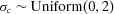
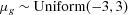
As an important component in Bayesian analysis, prior distribution should be properly selected. In this study, we use uniform distribution as priors to set a fairly large range for each parameter (including hyper parameters) but without specifying preference on any values in the corresponding range (i.e., flat prior, all values for each parameter in the corresponding range are equally likely). For the parameters a and b where the hierarchical structure is used, the hyper priors for the parameters in the lognormal distributions are specified as  ,
,  ,
,  , and
, and  . Based on Monte Carlo simulation, these settings allow parameter a to vary from 10−4 up to at least 1.3 × 10⁴ and b to be approximately in the range of (9 × 10⁻⁶, 3 × 10⁴). Using uniform distribution as a prior for variance parameters (e.g.,
  and
and  ) was proposed and discussed in Gelman et al.10 However, priors for e1 in Equation 2, and the parameters c and g with no hierarchical structure are specified as
  ,
,  , and
, and  . The proposed hierarchical model with prior specifications is graphically shown in Fig. 1.

For the purpose of comparison, some alternative hierarchical structures were also employed and the results obtained are compared with the ones from the proposed hierarchical model on partial parameters. When hierarchical structure is only used for a or b, uniform distribution is also specified as  and
and 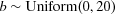 . When hierarchical structure is additionally placed on parameters c and g (i.e., the model presented in the Appendix), the hyper priors for the parameters are specified as
 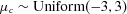 ,
,  ,
,  , and
, and  . Again, the main purpose of using uniform distribution as prior is to set a reasonable boundary on the parameters without giving any preferences. We also examined another flat prior option, normal distribution Normal(0, 10002) with the same lower and upper bounds corresponding to the uniform distributions, and we obtained almost identical estimates for the quantities of interest.
The proposed methods are programed in R (Version 3.3.1) using RStan.18 The MCMC sampling process consisted three different Markov chains sampled for 20,000 iterations. The first half of each chain is disregarded as burn-in, which results in a posterior sample size of 30,000. The convergence of the MCMC sampling is judged by the potential scale reduction statistic,  19 provided in the output of RStan. The values of
  reported indicate that all chains converged.
3.3. Results
The posterior distribution of relative risk estimates at 10 μg/L is calculated using the posterior sample of model parameters. We focus on 10 μg/L as it is the US EPA's current regulatory standard as well as WHO's recommended limit on inorganic arsenic concentration in drinking water. The 5th, median, and 95th percentile of the relative risk estimates at the low-exposure level for the Hill model using the proposed hierarchical model are reported in Table II (listed as H-ab). For comparison purposes, the corresponding estimates for single study and alternative hierarchical structures are also calculated and listed in the table, including (1) no hierarchical structure on any parameters (i.e., H-0), (2) hierarchical structure only on parameter “a” (i.e., H-a), (3) hierarchical structure only on parameter “b” (i.e., H-b), (4) hierarchical structure on all model parameters (i.e., H-all), (5) single data set from Sohel et al. (i.e., S-1), and (6) single data set from Chen et al. (i.e., S-2). In addition to the Hill model, the same quantities assessed using the linear model  , and the Power model,
  are provided in Table II. The WAIC values were calculated for the alternative hierarchical models and reported in Table II as well. In addition, the PPPs for the various combinations of model/hierarchical structure are reported in Table III and a description on how the PPPs were calculated is provided in the table caption.
| Hill Model | Power Model | Linear Model | ||||||||||
|---|---|---|---|---|---|---|---|---|---|---|---|---|
| 5th | 50th | 95th | WAIC | 5th | 50th | 95th | WAIC | 5th | 50th | 95th | WAIC | |
| H-ab | 1.000 | 1.118 | 1.418 | 73.07 | 1.006 | 1.086 | 1.631 | 65.93 | 1.008 | 1.259 | 2.520 | 67.16 |
| H-0 | 1.000 | 1.118 | 1.330 | 73.44 | 1.006 | 1.019 | 1.035 | 65.11 | 1.003 | 1.006 | 1.009 | 66.25 |
| H-a | 1.000 | 1.132 | 1.309 | 73.22 | 1.004 | 1.026 | 1.406 | 65.57 | 1.001 | 1.007 | 1.152 | 66.36 |
| H-b | 1.000 | 1.089 | 1.315 | 72.44 | 1.007 | 1.034 | 1.298 | 65.26 | 1.007 | 1.122 | 2.075 | 67.13 |
| H-all | 1.000 | 1.021 | 3.392 | 74.54 | 1.002 | 1.100 | 16.47 | 65.95 | – | – | – | – |
| S-1 | 1.000 | 1.086 | 1.273 | – | 1.004 | 1.017 | 1.032 | – | 1.002 | 1.005 | 1.008 | – |
| S-2 | 1.000 | 1.091 | 1.506 | – | 1.004 | 1.027 | 1.067 | – | 1.002 | 1.010 | 1.021 | – |
- Note: H-0 represents the model has no hierarchical structure on any parameters; H-a and H-b represents hierarchical structure only on parameter “a” or “b”, respectively; H-ab represents the model with hierarchical structure on both “a” and “b”; H-all has hierarchical structure on all model parameters; S-1 and S-2 are single data sets from Sohel et al. and Chen et al., respectively. WAIC was calculated to compare various hierarchical models, but not for individual studies. For the linear model, the H-ab model is the same as the H-all model, so the estimated values are not reported for H-all.
| Hill Model | Power Model | Linear Model | ||||
|---|---|---|---|---|---|---|
| S-1 | S-2 | S-1 | S-2 | S-1 | S-2 | |
| H-ab | 0.219 | 0.201 | 0.067 | 0.116 | 0.143 | 0.061 |
| H-0 | 0.333 | 0.234 | 0.066 | 0.088 | 0.704 | 0.805 |
| H-a | 0.122 | 0.077 | 0.062 | 0.109 | 0.100 | 0.089 |
| H-b | 0.223 | 0.211 | 0.059 | 0.027 | 0.139 | 0.180 |
| H-all | 0.313 | 0.141 | 0.071 | 0.097 | – | – |
| Single | 0.499 | 0.613 | 0.008 | 0.109 | 0.136 | 0.167 |
- Note: The posterior predictive p-value (PPP) is calculated using the method described in Gelman et al.:10
 , that is, the probability that the test statistic
  calculated using observed data is larger than the same statistic obtained using predicted data. In our case, the test statistic is the log-likelihood estimated based on the assumed Poisson distribution. y and ypred represent, respectively, the observed data (e.g., case numbers) and predicted case numbers, which were generated using the posterior sample of estimated parameters. Under a Bayesian framework, the probability can be numerically approximated by counting the number of sets of posterior samples that satisfy the inequality out of the entire posterior sample space. Using such a method, a very large or very small PPP means that it is very likely to see a discrepancy in predicted data, further indicating a poor fitting. Therefore, a PPP value within the range from 0.05 to 0.95 indicates an adequate fit. For the linear model, the H-ab model is the same as the H-all model, so the PPP values are not reported for H-all.
From the tables, we can find that the Hill model has higher PPP values (indicating a better fit) and WAIC values (posterior predictive density adjusted for overfitting, indicating a nonfavorable model selection) than the Power and linear models.
There are two main reasons for this result: (1) the Hill model with four parameters has a more flexible shape to fit the data than the Power and linear models, which do not fit the data well, and, (2) as the model has four parameters and there are a limited number of exposure groups, the variation in the posterior sample of the Hill model make the WAIC value higher than the Power and linear models. As demonstrated by the Power and Linear models, the distribution of estimated relative risk is wider (mainly the upper bound is higher) than the counterpart estimated from a single population in a study. As shown in Table II, the distribution of relative risk estimated from the hierarchical structure on the Hill model is smaller than the corresponding value estimated from the single Chen et al. study. The reason again is that the limited data points increased the estimation uncertainty for the Hill model, but when studies are allowed to share information through the hierarchical structure, this uncertainty is reduced.
4. SIMULATION STUDY
We propose a simulation study to test if the hierarchical structure on partial model parameters can adequately quantify the variability in relative risk with a focus on low exposures and investigate the effect of the number of studies on the estimate of population variability.
4.1. Study Design
We again use the fundamental assumption that the human variability is jointly caused by two factors: the variability in risk at background exposure and in the sensitivity of human response, which can be explicitly represented by the two parameters in the linear model, the model chosen to serve as the “true” model for simulating data sets. As this study focuses on examining how well the proposed hierarchy can quantify the variability over the background and slope of the response, the linear model is chosen to avoid introducing uncertainty and variability represented by other model parameters. In the simulation study, some modeling assumptions and settings used in the above data analyses can be simplified and will be explained in detail in the description of the simulation study below.
The linear model  , with the distributions:
  and
and  (exposure d is on a normalized scale, i.e., between 0 and 1), is used to generate exposure-response data to describe the relationship between arsenic concentration and relative risk. The reason to use these two specified distributions for the model parameters is that the resulting relative risks of death from cardiovascular diseases associated with arsenic exposure through drinking water are compatible to the values reported in recent epidemiological studies.15-17, 20 As the relative risk is a measurement calculated based on groups of subjects, each specified linear curve quantifies the relationship in a population (i.e., all subjects in a study) and the prescribed distributions of a and b are used to characterize the variability across populations (i.e., across studies). With the known distribution of model parameters and model settings, we can use extensive Monte Carlo simulation to accurately approximate the distribution of relative risk at any exposure. The process of the entire simulation study is: we first simulate a large number of study data sets from this true curve with known interpopulation variability, then use the hierarchical structure on partial parameters proposed in this study to quantify the variability, and finally compare with the known distribution to determine the accuracy of the proposed method.
The exposure level, relative risk, and observed cases are simulated to form simulation data sets. We assume that there are five exposure groups in the range of 0–400 μg/L in each study. These five groups are separated as: 0–10 μg/L, 10–50 μg/L, 50–100 μg/L, 100–200 μg/L, and 200–400 μg/L. The five exposure levels in each study are independently and randomly generated from these five uniform distributions specified by these five intervals. Exposure levels are then transformed to the (0, 1) interval by dividing by 400.
To simulate relative risk, values of “a” and “b” are randomly sampled from the true lognormal distribution [i.e.,  and
and  ]. Then, this pair of parameter values and the exposure vector are used to calculate the relative risks for the five exposure groups by using the linear model
  , which ensures that the relative risk is equal to 1 at the 0 exposure level (rather than at the lowest exposure group commonly reported in epidemiological studies).This relative risk,
  is used to generate a randomized relative risk as
  . We consider three different situations: (1) no randomness (i.e.,
 ) in the relative risk; (2) small randomness (i.e.,
  ); and (3) large randomness (i.e.,
  ). This variance parameter basically represents the randomness caused jointly by the interindividual and interpopulation heterogeneity. When σ is 0, it means that interpopulation variability can be perfectly described by the “true” linear model with specified distributions of parameters. However,
  means that great additional interpopulation and interindividual variability have been incorporated in the simulated relative risk values.
-
Generate 1,000 values from a lognormal distribution LogNormal(3.5, 1.5) (where 400 μg/L is higher than the 95th percentile).
-
Bin these subjects into previously specified exposure groups, i.e., 0–10, 10–50, 50–100, 100–200, and 200–400 μg/L and count the number of cases in each group,
 .
. -
Draw the number of cases randomly from a Poisson distribution with mean equal to
 for each exposure group to form the last vector in a simulated data set, the observed cases,
  .
.
The first step takes sampling variability into account. The number of values generated from the lognormal distribution (i.e., the sample size) is closely related to the sampling variability. The larger the sample size is, the more certain the proportion of the sample size of each group is (i.e., the smaller the sampling variability among exposure groups is). The reason to choose 1,000 is that it is close to the total number of observed cases in Sohel et al.,15 one of the studies analyzed in Section 3.. The last step above to generate observed case number from a Poisson distribution is essentially building individual-level uncertainty and variation in the simulated data sets. That is, greater relative risk value leads to higher variation in the simulated number of observed cases, and this is aligned with the common situation that larger variation is usually observed in the highest exposure group. The following two vectors are two exemplary sets of observed case numbers generated through this process: [219, 495, 250, 312, 261] and [190, 456, 121, 158, 93]. We need to point out that the number of cases in each exposure group basically determines how much weight this data point (i.e., this exposure group) contributes to the model fitting process; therefore, the distribution of the cases among exposure groups is more directly related to the model fitting than the total sample size.
These three vectors together can form a complete simulation data set for exposure-response modeling, but the model approach is slightly different from the one stated in the previous section. The main reason for the difference is that the expected number of cases in each exposure group in the simulation study is independently generated rather than estimated based on the assumption that supports Equation 2. Therefore, the expected cases can be simply calculated from the observed data vector and the relative risk vector as  and substituted for the corresponding parts in Equation 3 for model parameter estimation. The simulation considers three scenarios. The first scenario is that each set of studies includes two simulated data sets representing two different populations. Then, the proposed hierarchical structure is applied to quantify interpopulation variability via the Hill model, Power model, and linear model. The remaining two scenarios have five studies and eight studies being included for hierarchical modeling, respectively. Five hundred sets of studies are used in each scenario, so, for instance, for the two-study scenario, 1,000 different data sets were simulated, while 4,000 data sets were randomly generated in total for the eight-study scenario.
The “true” distribution of relative risk at a given exposure is characterized by Monte Carlo simulation. From the distribution  and
and  previously specified, 100 million samples were generated for “a” and “b” each. For the exposure at level 10 μg/L, 100 million values of relative risk
  can be calculated. These 100 million values are further used as the median in the lognormal distribution to simulate 100 million relative risk
  for each of the three situations: no randomness (NR), small randomness (SR), and large randomness (LR). We believe that the 100 million samples can quite accurately characterize the distribution of the relative risk, and therefore the median and 95th percentile estimated from the 100 million sample are used as “true” value. For example, at 10 μg/L, the true median and 95th percentile of relative risk for all three situations is 1.0679 and 1.2494 (for NR), 1.0774 and 1.2725 (for SR), and 1.0879 and 1.6756 (for LR).
4.2. Results
 (7)
(7)The mean and standard deviation of the log ratio of the median and 95th percentile based on the 500 repetitions for each model/scenario combination are listed in Table IV for all three situations considered. The 500 log ratios for each combination are also graphically shown in Figs. 2–4 for the three situations.
| Median | 95th Percentile | ||||||
|---|---|---|---|---|---|---|---|
| 2 Studies | 5 Studies | 8 Studies | 2 Studies | 5 Studies | 8 Studies | ||
| NR | Hill | −0.0042 | −0.0019 | −0.0019 | 0.4429 | 0.2469 | 0.1471 |
| (0.0321) | (0.0219) | (0.0166) | (0.2088) | (0.1894) | (0.1415) | ||
| Power | 0.0003 | 0.0015 | 0.0011 | 0.4899 | 0.2469 | 0.1471 | |
| (0.0338) | (0.0225) | (0.0172) | (0.2147) | (0.1950) | (0.1451) | ||
| Linear | 0.0014 | 0.0020 | 0.0014 | 0.4891 | 0.2453 | 0.1463 | |
| (0.0334) | (0.0226) | (0.0171) | (0.2127) | (0.2004) | (0.1455) | ||
| SR | Hill | −0.0113 | −0.0102 | −0.0106 | 0.4372 | 0.2127 | 0.1180 |
| (0.0344) | (0.0225) | (0.0173) | (0.2307) | (0.1930) | (0.1454) | ||
| Power | −0.0064 | −0.0064 | −0.0071 | 0.4905 | 0.2373 | 0.1345 | |
| (0.036) | (0.0235) | (0.0179) | (0.2339) | (0.2002) | (0.1502) | ||
| Linear | −0.0073 | −0.0069 | −0.0074 | 0.4720 | 0.2304 | 0.1312 | |
| (0.0338) | (0.0224) | (0.0171) | (0.2110) | (0.2028) | (0.1475) | ||
| LR | Hill | −0.0167 | −0.0160 | −0.0178 | 0.0952 | −0.0596 | −0.1253 |
| (0.0770) | (0.0526) | (0.0401) | (0.5262) | (0.3083) | (0.2232) | ||
| Power | 0.0056 | −0.0011 | −0.0060 | 0.3010 | 0.0388 | −0.0617 | |
| (0.0763) | (0.0518) | (0.0390) | (0.4876) | (0.2974) | (0.2220) | ||
| Linear | −0.0142 | −0.0142 | −0.0153 | 0.2108 | −0.0145 | −0.0998 | |
| (0.0377) | (0.0265) | (0.0200) | (0.2221) | (0.2074) | (0.1638) | ||
- Note: The standard deviation for each model/number of studies combination is provided in parentheses. NR, no randomness; SR, small randomness; LR, large randomness.


The results show that as the number of studies included increased, both the median and 95th percentile estimates are closer to the true value, and the variance in the estimates decrease. The majority of the log ratios are positive, indicating that the estimated values are typically larger than the true value. For the 95th percentile, higher estimated value is acceptable because the higher value will usually lead to a more conservative regulation on the exposure. As shown in both Table IV and Figs. 2–4, the Power model and Hill model can generally provide estimates as adequate as the linear model even if it is the true model used to generate data sets.
5. CONCLUSION AND DISCUSSION
As suggested by both the simulation study and application to real data, the proposed hierarchical model on partial model parameters can be used to adequately quantify variability across different populations.
The proposed hierarchical model on partial parameters focuses on quantifying the variability via quantifying the distribution in risk at background exposure and the sensitivity of response, which are the two main factors that are mostly relevant to the variability in responses at low exposures. However, we need to note that the sensitivity of response in the Hill model (Equation (4)) may not be precisely represented by the parameter “b” solely if we define the sensitivity of response as the first derivative with respect to dose, which is  . In other words, the sensitivity of response may be jointly characterized by all three other parameters in the Hill model except the background parameter “a.” Therefore, we also investigated the hierarchical structure over all of the four parameters in the epidemiological data application (in Tables II and III) and simulation study (in the Appendix). Given these results in Table II, we can find that the 95th percentile of relative risk estimated from the “H-all” model is higher than the one estimated from the “H-ab” model. Meanwhile, the log-ratio of the 95th percentile of the “H-all” model in the two-study situation displayed in Fig. A.1 is much higher than its counterpart estimated using the “H-ab” model. These two pieces of evidence demonstrate that when the number of studies included in an analysis using a hierarchical model is small, the width of the 90th percentile interval can be significantly affected by the number of parameters with a hierarchical structure. On the other hand, when there are sufficient studies included in an analysis using a hierarchical model (i.e., the five- and eight-study cases in Fig. A.1), the difference in the results estimated from the two hierarchical structures is very limited. Therefore, it is not necessary to build a full hierarchical structure on all model parameters when we only focus on the low-exposure range. One reason for using the partial model is that, when we focus on the human data in low exposure, it is very likely that the dose is very small (relative to parameter “c”), and parameter “g” is often close to 1, which makes the derivative (i.e., the sensitivity of response) mainly depend on “b.” The similar results of the five- and eight-study situations shown in Fig. A.1 well support this argument. Another advantage of the proposed hierarchical structure on the parameters of interest (i.e., “a” and “b”) is that this method is less model dependent, which has a two-fold meaning. First, most of the exposure-response models contain the two parameters representing the background and sensitivity. Second, as shown in Tables II and IV, the hierarchical structure on partial parameters provides quite similar distribution estimates of relative risk in various situations examined regardless of the format of exposure-response models.

The available exposure groups in the studies being analyzed has a very important impact on model selection and the variability quantification. As suggested by the data analysis results in Section 3.3., insufficient data points (number of exposure groups smaller than the number of model parameters) can introduce significant estimation uncertainty into the final estimates of variability in relative risk. However, models with more parameters (e.g., the Power model and Hill model) are more flexible to fit various shapes of exposure-response relationship. In addition, more model parameters make the estimates at low exposure levels more resistant to the disturbance caused by the responses at high exposure levels. As shown in the simulation study (Table IV), the accuracy of the linear model is generally no better than the Power model or Hill model, even if the linear model is the “true” model for generating simulation data sets. But again, the selection of exposure-response models is largely limited by the available number of exposure groups.
The results suggest that as the number of studies increases, the uncertainty in estimates decreases. When the number of studies is small, the estimated distribution is wider than the true distribution. From a conservative perspective, a limited number of studies will not hurt risk assessment. Theoretically, to include more studies is always beneficial for increasing the accuracy of estimation, but the improvement in accuracy is clearly reduced when the number of studies included reaches five. This suggests that to balance the cost and the effectiveness of reducing uncertainty and improving accuracy, five studies might be a good option. However, we need to note that we assumed each data set had five exposure groups in the simulation study, so it should be expected that more studies are needed when fewer exposure groups are contained in each study.
Prior and hyper prior distribution can have potentially large impacts on the distribution estimation, that is, wider prior distribution may lead to wider distribution of the relative risk estimates. In this study, we examined two possible options of flat prior, the uniform distribution and truncated normal distribution with very large variance, to set a boundary on the model parameters. Because such settings on boundaries were kept identical in various situations and scenarios we examined, the results of comparison are robust to the prior specifications. However, priors should be carefully selected and tested for sensitivities in practice.
Finally, we also need to note that what has been focused on in this study is the interpopulation variability, which is only a part of the interhuman variability. When data are only available at the population level like the examples we employed in article, the hierarchical model is useful to probabilistically quantify the variability among different populations. However, if more detailed information regarding pharmacokinetic and/or pharmacodynamics in humans is available, variability at the individual level also should be incorporated and quantified.3 One source of uncertainty not considered in this study is exposure uncertainty, which is an important but difficult factor in exposure-response assessment using epidemiological data. In our next study, we will focus on investigating how exposure uncertainty will influence the variability and uncertainty in risk estimates.
ACKNOWLEDGMENTS
This research is partially supported by Indiana University School of Public Health Developmental Research Grants for Pre-Tenure Faculty. The authors thank Drs. Jeffrey S. Gift and Woodrow Setzer and anonymous reviewers for their comments on earlier versions of the article.
APPENDIX A

 and
and  are both assumed to be lognormal distributions. For the hyper parameters
  , and
, and  , we assume that these parameters are independent a priori, and place a uniform prior same as the corresponding ones for parameter “b” in Equation 6. All the remaining parameters have the same meaning as in Equation 6. This model structure was also employed in the simulation study. Similarly, the mean and standard deviation of the log ratio of the median and 95th percentile estimated from this model are listed in Table A.I. In addition, the log ratios estimated from the “H-ab” and “H-all” structures of the Hill model are compared and graphically shown in Fig. A.1 in the Appendix.
| Median | 95th Percentile | ||||||
|---|---|---|---|---|---|---|---|
| 2 Studies | 5 Studies | 8 Studies | 2 Studies | 5 Studies | 8 Studies | ||
| NR | Hill-all | −0.0147 | −0.0037 | −0.0026 | 0.9611 | 0.2439 | 0.1346 |
| (0.0293) | (0.0218) | (0.0167) | (0.2705) | (0.1869) | (0.1423) | ||
| SR | Hill-all | −0.0234 | −0.0128 | −0.0119 | 0.9807 | 0.2555 | 0.1272 |
| (0.0315) | (0.0226) | (0.0172) | (0.2732) | (0.1911) | (0.1441) | ||
| LR | Hill-all | −0.0433 | −0.0484 | −0.0525 | 1.1954 | 1.1302 | 1.1651 |
| (0.0546) | (0.0403) | (0.0303) | (0.6287) | (0.7414) | (0.7194) | ||