Against all odds: Harbor porpoises intensively use an anthropogenically modified estuary
Abstract
Harbor porpoises (Cetacea) are present in the North Sea throughout the year but periodically enter adjacent estuaries, which due to human activities are among the planet's most threatened aquatic systems. However, the occurrence of harbor porpoises in estuaries has rarely been studied. In this work, harbor porpoise occurrence at two stations in the anthropogenically modified Ems Estuary (Germany, Netherlands) was modeled using a machine learning approach (Random Forest) that drew on 8 years of acoustic monitoring data with C-PODs together with environmental data. Harbor porpoises were present year-round at both stations. According to the models, their detection was mainly explained by season, tide, and noise level, with the highest detection probabilities in spring, at high tide, and at low noise levels. The seasonal and tide-dependent occurrence of harbor porpoises coincided with prey availability. Presumed feeding activity was detected in 47% of all harbor-porpoise-positive 10 min blocks and indicated the importance of the estuary as a regular feeding area. The elevated noise levels detected at one station were attributed to tidal-induced currents and sediment movements. The results of this study can help to improve estuarine management through measures that include conducting dredging and disposal activities when harbor porpoise occurrence is less likely.
1 INTRODUCTION
Harbor porpoises (Phocoena phocoena) are small odontocetes that are common in the North Sea (Hammond et al., 2013), where their density is estimated to be 0.52 animals/km2 (Hammond et al., 2017). In the southwestern part of the German North Sea, increasing densities of harbor porpoises have been reported over the last decade (Peschko et al., 2016). Harbor porpoises are top-predators and in the North Sea they mainly feed on small pelagic and demersal fish, such as clupeids, sand eels, roundfish, gobies, gadoids, and flatfish, with seasonal and age-dependent variations (Leopold, 2015; Santos & Pierce, 2003). Due to their energy requirements, harbor porpoises must forage nearly continuously, which makes them particularly vulnerable to environmental disturbances (Wisniewska et al., 2016; but see also Hoekendijk et al., 2018 and Wisniewska et al., 2018).
Harbor porpoises almost exclusively rely on echolocation (biosonar) for orientation (Verfuss et al., 2005), prey capture (Miller, 2010), and communication (Clausen et al., 2010). They emit narrow-band high-frequency (NBHF) signals (so-called clicks) between 110 and 160 kHz (Villadsgaard et al., 2007), with a peak frequency between 125 and 140 kHz (Au et al., 1999). The click rate, and thus the interclick interval (ICI), can be adjusted depending on the target to between <10 ms and 250 ms (Wisniewska et al., 2012). When a harbor porpoise approaches a prey item, the ICI is around 50 ms, decreases progressively to <1.5 ms at a distance of 2–4 m to the prey, and ends in a terminal “buzz” when the prey is captured (Miller, 2010). Usually, click sequences with an ICI <10 ms are considered to indicate feeding behavior (e.g., Nuuttila, 2013; Todd et al., 2009; Zein et al., 2019). The biosonar behavior of harbor porpoises can be exploited in the acoustic detection of these animals in their natural habitat; consequently, harbor porpoise occurrences have often been studied using passive acoustic monitoring (PAM) devices (e.g., Nuuttila et al., 2018; Pirotta et al., 2014; Wenger & Koschinski, 2012; Zein et al., 2019).
North Sea harbor porpoises regularly enter adjacent estuaries (Weel et al., 2018; Wenger & Koschinski, 2012), which represent transition zones between the river and the sea. Estuaries are characterized by a longitudinal salinity gradient that determines the structural features of their biota (Elliott & Whitfield, 2011; Taupp & Wetzel, 2014) and they are among the most productive environments worldwide (Whittaker & Likens, 1973). However, estuaries are also one of the most threatened and modified aquatic systems, due to human activities and disturbances such as fairway deepening, the dredging and disposal of sediments, harbor and marina operations, shipping, diking and impoundment, tourism and other recreational activities, the discharge of pollutants, and nutrient enrichment (Beineke et al., 2005; Blaber et al., 2000; Das et al., 2004; Kennish, 2002). This has led to losses of habitat and species diversity, the alteration of organismal communities, and an increase in species invasions (Lotze et al., 2006; Taupp & Wetzel, 2019). Consequently, the estuary conditions supporting cetaceans have changed as well. In addition, harbor porpoises are prone to other types of anthropogenic disturbances common to oceans and estuaries, such as noise (Duarte et al., 2021; Erbe et al., 2019; Todd et al., 2015).
Estuaries usually represent the border area of harbor porpoise distribution such that the abundance of these animals in this habitat is lower than in the sea. This may explain why harbor porpoises in estuaries have long been neglected by researchers. However, knowledge about the use of estuaries by these marine mammals is important for management and conservation because all cetaceans are protected under European law as species of community interest in need of strict protection (Council Directive 92/43/ EEC of 21 May 1992 on the conservation of natural habitats and of wild fauna and flora, Annex IV). Yet for German estuaries, studies of the long-term impact of environmental factors on harbor porpoises are lacking. To fill this gap, in this study PAM data from two stations in the Ems Estuary collected over an 8-year period (from April 1, 2012, to March 31, 2020) were used in a machine learning approach to fit models of harbor porpoise occurrence as a function of environmental variables. In addition, the relative importance of the predictors of harbor porpoise occurrence identified by the models was determined and the predictor-response relationships based on the model's predictions were assessed.
2 MATERIAL AND METHODS
2.1 Study site
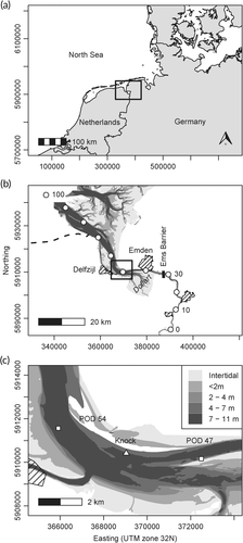
The coastal-plain Ems Estuary is located at the southern coast of the North Sea, close to the Dutch border (Figure 1). The Ems drains a catchment area of 17,934 km2 into the Wadden Sea (Krebs & Weilbeer, 2008), an area encompassing North Sea coastal zones in southern Denmark, Germany, and the northern Netherlands (Common Wadden Sea Secretariat, 2010). The lower section of the estuary has a typical funnel shape but also a conspicuous morphological feature, the so-called Dollart, a tidal basin of about 100 km2 (ca. between river-km 32 and river-km 43) that presumably formed as a result of flood events in the Middle Ages. The median freshwater discharge is ~60 m3/s and the mean tidal range ~2.25 m. Salinity follows a distinct longitudinal gradient (Krebs & Weilbeer, 2008). The estuary serves as the seaway to the German seaport at Emden (located ca. at river-km 41) and to the Dutch seaport at Delfzijl (ca. river-km 56) and has thus been under anthropogenic pressure for decades, among other reasons due to ship traffic; port, dyke, and floodgate construction; and fairway deepening (van Maren et al., 2015). In the study area, vessel density based on AIS data (Universal Shipborne Automatic Identification System), averaged from 2012 to 2017, ranged between 30 and 50 vessels per km2 per day (Bundesamt für Seeschifffahrt und Hydrographie, 2020). To maintain the fairway depth, the mean annual dredged volume during the same period was 6.68 ± 0.93 million m3 (mean ± SD) between river-km 30 and river-km 113. Dredging was done year-round, and the material was brought to disposal sites within the estuary (Waterways and Shipping Office, Emden, personal communication, June 2020). This and other activities have converted the Ems Estuary into a hyperturbid system (Winterwerp et al., 2013) characterized by thick layers of fluid mud (Leussen, 2011).
2.2 Field methods
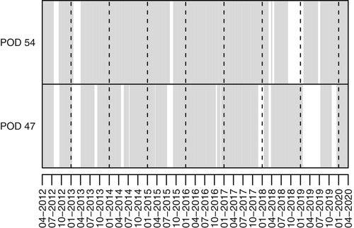
Harbor porpoise occurrence was examined using C-PODs (Cetacean Porpoise Detectors; Chelonia Ltd., UK; https://www.chelonia.co.uk). C-PODs are self-contained acoustic data-loggers that use an omni-directional hydrophone (20–160 kHz) to register the echolocation clicks of odontocetes, recording the time, duration, frequency, sound pressure level, duration, and bandwidth of each click. C-PODs are able to record only a limited number of clicks per minute (4,096). If this limit is exceeded, e.g., due to high background noise, the remaining timespan within this minute without recording is internally stored as “percent time lost.” According to the manufacturer, the maximal detection range of the C-POD for porpoise clicks is approximately 300 m. However, the effective detection range depends on various factors, such as tidal flow, water depth, current speed, and ambient noise, and thus varies between approximately 100 and 450 m (Nuuttila et al., 2018). The acoustic detection probability of harbor porpoises also depends on other factors, such as the source level of their clicks, which can differ between habitats (Kyhn et al., 2013); acoustic activity, which may be reduced under noisy conditions (Brandt et al., 2011); and beam directionality (Macaulay et al., 2020). In this study, C-PODs were deployed at river-km 47 (POD 47) and river-km 54 (POD 54) close to the fairway (Figure 1). The lowest astronomic tide (LAT) is ca. 5.5 m at POD 47 and ca. 7.5 m at POD 54. Each C-POD was moored at a steel rope connected with an anchor stone and buoyancy bodies ca. 1 m (POD 47) and ca. 2.5 m (POD 54) aboveground (Walter et al., 2011). The data of these C-PODs were analyzed from April 1, 2012, to March 31, 2020 (2,922 days). Data gaps occurring within this 8-year period were due to device failure or the removal of the C-PODs from the water during ice conditions (Figure 2). Thus, recordings were obtained for 2,361 days at river-km 47 (80.8% of the entire study period) and 2,567 days at river-km 54 (87.9%). The high-pass filter of the C-PODs was set to 80 kHz (default 20 kHz) to take into account the high levels of background noise determined in preliminary analyses of C-POD data. From April 2018 onwards, the C-POD sensitivity was set to “low sensitivity” to exclude weaker clicks and reduce the amount of recorded background noise. At each of the two positions, after an operating time of 1–3 months, the C-PODs were switched out for new ones, mooring was controlled, batteries were replaced, biofouling was removed, and data from the SD cards of the C-PODs were copied to a notebook using the software CPOD.exe provided by the manufacturer.
2.3 Processing of C-POD data
C-POD data were processed using CPOD.exe, version 2.044. Potential click sequences (trains) of harbor porpoises were filtered using the built-in train detection algorithm KERNO-classifier, with the quality class settings “high” (very likely to come from a source of click trains) and “moderate” (likely to come from a source of click trains) in accordance with other studies in similar environments (e.g., Rodrigues, 2014; Zein et al., 2019). The parameter “species” was set to “NBHF” (narrow-band high frequency), which ensured that only species producing NBHF clicks, such as all Phocoenidae, were considered. The results of the train detection algorithm were analyzed within 10 min blocks. Each block in which the algorithm detected at least one harbor porpoise train was checked manually for false positives arising, for instance, due to background noise. The manual control followed the guidelines of the manufacturer (https://www.chelonia.co.uk) and Gallus et al. (2012), who used PODs in the Baltic Sea, a low-density area where manual control is generally suggested as good practice (see also Amundin, 2016). Manual control particularly considered amplitude profile, inter click interval, frequency, number of cycles, and the coherence of the clicks. If at least one true detection was present within a 10 min block, this block was defined as harbor-porpoise-positive 10 min. If the ICI of at least one porpoise click sequence fell below 10 ms, this block was considered to indicate feeding behavior. Subsequently, the percentage of these blocks indicating feeding behavior in relation to all harbor-porpoise-positive 10 min blocks was calculated.
2.4 Processing of environmental data
For each 10 min block, water temperature data were obtained from the built-in temperature sensor of the C-POD. The water level was measured continuously at the Knock gauging site, which is operated by the Waterways and Shipping Office and located at river-km 50.9, between the two C-POD stations (Figure 1). The date and time of every high tide within the study period were determined. Subsequently, for the timepoint in the middle of each 10 min block the temporally closest high tide and the respective difference in hours was calculated, resulting in values from ~ − 6 hr to ~ + 6 hr. Oxygen concentration and turbidity were measured at the same gauging site, with missing data estimated using a dynamic time warping algorithm (Phan et al., 2020). For each date and C-POD position, the sunrise and sunset times were determined using algorithms provided by the National Oceanic and Atmospheric Administration (https://www.noaa.gov). For each day, sunrise and sunset data were standardized to values between 0 and 1 for the time between sunrise and sunset (day) and between 1 and 2 for the time between sunset and sunrise (night), using the timepoint in the middle of each 10 min block. To include the effect of background noise, the parameter “nall” in CPOD.exe, averaged for each 10 min block, was used, as also described in Nuuttila et al. (2018). The parameter nall is derived from the unfiltered data file and contains all recorded clicks within the frequency range of the C-POD. According to the manufacturer, potential click sources besides cetaceans that contribute to nall include sonars, pingers, shrimp, fish finders, sediment movement noise, ship traffic, and current noise.
2.5 Statistical analysis
Harbor porpoise occurrence was predicted using Random Forest (RF), a machine learning approach based on unpruned regression or classification trees that enables supervised and unsupervised learning (Breiman, 2001). In this work, RF was run in the classification mode because the response variable (harbor porpoise occurrence) was binary (no/yes). RF was an appropriate choice as a modeling technique because (1) it has a very high classification accuracy, (2) it makes no assumptions regarding the distribution of variables, (3) it is able to model nonlinear data, (4) it handles complex interactions among predictors (Crisci et al., 2012; Cutler et al., 2007; Ryo & Rillig, 2017; Thessen, 2016), and (5) it provides importance-ranking methods for the predictors. Comparisons with other classification methods have shown that RF is an exceptionally good classification technique (e.g., Bučas et al., 2013; Chambault et al., 2021; Fernández-Delgado et al., 2014; Marini et al., 2015) and it has been successfully used in acoustic cetacean studies for different purposes, e.g., to predict bottlenose dolphin distribution as a function of environmental variables (Marini et al., 2015) and to determine the environmental variables that influence the acoustic occurrence of Antarctic blue whales (Shabangu et al., 2017).
In RF, a random bootstrap sample (sampling with replacement) of the original data is used to train a tree model. In each tree, a subset of predictor variables is randomly chosen and at each node the best split is selected. The number of predictor variables in this subset can be changed by the user by setting the parameter “mtry” (default value: square root of the number of predictor variables). In RF, this procedure of random bootstrap sampling and tree building is repeated a number of times (default value: 500 trees). Each decision tree returns a binary classification result and the class with the most votes is the final prediction of the model. Data not included in the bootstrap sample (typically about one-third of the original data) are referred to as out-of-bag (OOB), and each OOB data set is used to check the model, i.e., the trees are run with the OOB samples. The proportion of incorrectly classified OOB samples is the OOB error.
The following 11 predictor variables were used for RF modeling (abbreviations used throughout the paper are given in parentheses): temperature (temp), day of the year (dayNr), year (year), hour of the day (hour), standardized daytime depending on sunrise and sunset (dayTime), time from/to the temporally closest high-water level (tchw), oxygen concentration (o2), turbidity (turb), number of all recorded clicks (nall), percent time lost (timeLost), and the low sensitivity C-POD setting (lowSens). Additionally, a random number variable (0–100, uniform distribution) was added to eliminate unimportant predictors (details provided below). The response variable was harbor porpoise occurrence (no/yes).
For each of the two PODs, a separate RF classification model was calculated to enable better model interpretation despite the background noise, because the nall values of POD 54 were about six times higher than those of POD 47. The data set of each C-POD was split into a training data set (70% of the samples) and a test data set (30% of the samples) such that the no/yes ratio of the response variable was kept constant. The two classes of the response variable were highly imbalanced at both stations (POD 47 and POD 54: yes: 1%, no: 99%), which could have had a serious negative impact on model fitting (Chen et al., 2004). This was taken into account by subsampling the training data set by undersampling the majority class (Menardi & Torelli, 2014), after which the RF was applied to the undersampled training data set (POD 47 and POD 54: yes: ~50%, no: ~50%). Based on the resulting model, variable importance was calculated as the mean decrease in the area under the curve (Ballings & Van den Poel, 2016) and the response variable of the test data set was predicted. The model's performance was evaluated by calculating the confusion matrix, sensitivity (true positive rate), specificity (true negative rate), and receiver operating characteristics (ROC) curve, with the latter used to calculate the area under the curve (AUC). The value of the AUC is 0.5 when the model performs not better than chance and 1 if the classifier predicts all values correctly. The model's complexity was reduced by discarding all predictors with less importance than the random number variable (Becker et al., 2020; Eguchi et al., 2017). For each RF model, tuning was done by setting mtry to values of 2, 3, or 4 and then manually selecting the value that resulted in the highest sensitivity and specificity of the test data set. For the final RF model, partial dependence plots of the three most important predictors were calculated. Partial dependence plots show the relative logit contribution of the predictor to the predicted class probability after the effects of all other predictors in the model have been averaged out (Cutler et al., 2007; Hastie et al., 2009). Associations between the three most important predictors of each model were visually controlled using density plots based on kernel density estimates and by fitting smoothed local polynomial regression lines to the plot. The smoothing parameter was chosen automatically via generalized cross-validation (Wang, 2010).
All statistical analyses were done in the R environment (R Core Team, 2017) using the following R packages: caret, version 6.0–85 (Kuhn, 2020), DTWBI, version 1.1 (Phan et al., 2020), fANCOVA, version 0.5–1 (Wang, 2010), maptools, version 0.9–9 (Bivand & Lewin-Koh, 2019), ROSE, version 0.0–3 (Lunardon et al., 2014), randomForest, version 4.6–14 (Liaw & Wiener, 2002), and interpretR, version 0.2.4 (Ballings & Van den Poel, 2016).
3 RESULTS
3.1 POD records
From the 709,307 10 min blocks recorded at the two stations, 9,375 (1.32%) were classified as harbor porpoise positive by the algorithm and hence manually checked. From the latter group of blocks, 1,971 (21.0%) contained one or more false-positives and no true positives (POD 47: 20.1%, POD 54: 21.8%), resulting in 7,404 harbor-porpoise-positive 10 min blocks (POD 47: 3,369; POD 54: 4,035). These data showed the year-round presence of harbor porpoises at both stations. Of these 7,404 blocks, 3,456 (46.7%) had at least one harbor porpoise click sequence with an ICI <10 ms, thus indicating feeding behavior (POD 47: 1,409; POD 54: 2,047). The median background noise (nall) was 183 for POD 47 and 587 for POD 54. The percentage of time lost (as a result of the click limit of the C-POD) was 2.51% for POD 47 and 15.80% for POD 54, indicating high levels of noise recorded at the latter station.
3.2 RF-model
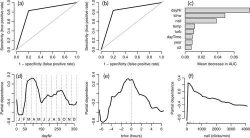
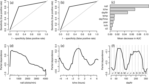
In the final RF-models for POD 47 and POD 54, the predictors hour, timeLost, and lowSens were excluded in the course of the variable elimination procedure. The AUC, sensitivity, and specificity for the two PODs ranged from 0.76 to 0.84 (Table 1, Figures 3a, b and 4a, b). The most important predictors for harbor porpoise occurrence were, in decreasing order, dayNr, tchw, and nall at POD 47 (Figure 3c), and nall, tchw, and dayNr at POD 54 (Figure 4c). In both models, dayNr showed a clear seasonal pattern, with the highest harbor porpoise occurrence probabilities from March to April, a decrease from May to June, another peak from July to October, and the lowest probabilities from November to February (Figures 3d and 4f). The model predictions for porpoise presence were highest for high tide (tchw, values of 0) both at POD 47 and at POD 54 (Figures 3e and 4e). Increasing nall values reduced the probability of harbor porpoise occurrence almost linearly (Figures 3f and 4d). For the remaining predictors (at both POD 47 and POD 54), probabilities were highest at temperatures from 6°C to 7°C, a turbidity of <0.5 g/L, an oxygen concentration from 7 to 10 mg/L, and during the night. Probabilities varied between years and stations, with the highest probabilities occurring in 2016 at both stations (Figures S1 and S2).
| AUC | Sensitivity | Specificity | ||
|---|---|---|---|---|
| Training data | POD 47 | 0.81 | 0.83 | 0.80 |
| Test data | POD 47 | 0.82 | 0.84 | 0.80 |
| Training data | POD 54 | 0.79 | 0.82 | 0.76 |
| Test data | POD 54 | 0.79 | 0.82 | 0.76 |
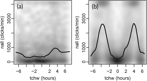
At POD 47, the predictors nall and tchw showed no clear dependencies (Figure 5a) whereas at POD 54, nall values were highest between high tide and low tide and lowest (around zero) at high tide and at low tide (Figure 5b). There were no clear dependencies between the other predictors with importance ranks between one and three (Figures S3 and S4).
4 DISCUSSION
This study of long-term data obtained from PAM showed that harbor porpoises use the Ems Estuary year-round. Detection probabilities were highest in early spring, at high tide, and at low noise levels. The high level of presumed feeding activity evidenced the importance of the estuary as a feeding area.
The day number (dayNr) was an important predictor of harbor porpoise occurrence in the RF-models, both at POD 47 and at POD 54. The partial dependence plots showed a clear seasonal pattern, with the highest values from March to April, high values from July to October, and lower values for the other months of the year. Previous studies also reported that the probabilities of harbor porpoise occurrence were highest in early spring, including studies using PAM in the outer Ems Estuary close to the Dutch coast in 2010 (Weel et al., 2018) and in the German Wadden Sea from 2012 to 2016 (Zein et al., 2019), studies based on sighting data in the Weser Estuary from 2007 to 2010 (Wenger & Koschinski, 2012), and aerial surveys of the Dutch continental shelf from 2010 to 2011 (Geelhoed et al., 2013). However, in the aerial surveys of the Dutch continental shelf from 2012 to 2017, the abundance estimates for spring were comparable to those of summer (Geelhoed & Scheidat, 2018). Aerial surveys in the German exclusive economic zone revealed a general seasonal movement pattern of harbor porpoises. The densities of harbor porpoises were highest in spring, lower in summer, and lowest in autumn, suggesting that the animals enter German waters in spring and leave them in autumn (Gilles et al., 2009). The distribution of harbor porpoises is generally closely linked to that of their prey (Gilles et al., 2016; Sveegaard et al., 2012) and the high detection rates in spring have been attributed to high fish abundances (e.g., Weel et al., 2018; Wenger & Koschinski, 2012; Zein et al., 2019). In the Ems Estuary, harbor porpoises may follow the anadromous fish that enter its waters in spring, such as the smelt (Osmerus eperlanus), which is an abundant species in the estuary (Kopetsch & Scholle, 2017). Smelt gather in the mouths of estuaries in winter, entering their waters in sizeable schools to spawn in spring (Vorberg & Breckling, 1999). Another abundant species in the Ems Estuary is the European sprat (Sprattus sprattus; Kopetsch & Scholle, 2017), which enters the coastal region in spring to spawn (Vorberg & Breckling, 1999). However, the most abundant fish species in the Ems Estuary is herring (Clupea harengus), specifically its juveniles, which use the estuary as a nursery ground. In September >90% and in May 60%–72% of all fish were herring (Kopetsch & Scholle, 2017). The clear decrease in the probability of harbor porpoise detections from May to June is consistent with the fact that these months correspond to the birth period of porpoises in the North Sea (Hasselmeier et al., 2004; Lockyer, 2007), when adult females leave the estuarine region and travel to the North Sea to give birth. In the North Sea, mating occurs in summer (Lockyer, 2007), after which harbor porpoises may return to the estuarine region of the Ems, at least in part because of the high fish abundance and biomass, mostly that of juvenile herring (Kopetsch & Scholle, 2017). In autumn, harbor porpoises again leave the estuary and German waters to feed elsewhere in the North Sea (Gilles et al., 2009).
Background noise (nall) was negatively and almost linearly associated with porpoise click detections and had a high importance ranking in the models. In general, this negative correlation suggests harbor porpoise displacement under noisy conditions or the masking of harbor porpoise signals by background noise. The latter may impede both automatic click detection by an algorithm and manual visual detections of recorded click sequences. In this study, masking was more likely because of the clear association of nall with the tide curve for POD 54, where nall values were highest between high tide and low tide. During this interval, current speed and suspended sediment concentrations in the estuary are highest (Ridderinkhof et al., 2000) and thus result in high levels of current and sediment transport noise. Consequently, harbor porpoise occurrence was likely to have been underestimated, especially at POD 54. At POD 47, background noise was of less importance (rank three) in the model compared with POD 54 (rank one); however, the harbor porpoise detection probability at POD 47 was also reduced when background noise was elevated. Why more sediment movement noise was recorded at POD 54 than at POD 47 is unclear but may have been due to differences in sediment grain sizes between the two C-POD stations. The sediment at POD 47 is mainly silty, whereas at POD 54 it mainly consists of fine sand, which is subject to intensive transport processes (German Federal Institute of Hydrology, unpublished data of sediment samples taken in 2015). However, differences in sediment movement noise between the two stations may also have reflected the estuary's complex and highly variable bathymetry and flows, also on a small scale (Pein et al., 2014). In most PAM studies that use models to describe harbor porpoise detections, the variable nall has not been used as predictor. However, it was included by Nuuttila et al. (2018) in their generalized additive model of harbor porpoise occurrence (1 hr blocks) in a bay in the United Kingdom. The results of that study identified nall as a significant predictor and its clear nonlinear relationship to porpoise clicks, which increased initially followed by fluctuations after a certain threshold. Future studies should consider the potential importance of background noise in acoustic monitoring of harbor porpoises and generally evaluate nall for inclusion as a variable in the respective models.
The tidal phase (tchw) was an important predictor at both stations, with highest detection probabilities at high tide. At POD 54, the tidal effect was likely to be at least partially masked by the background noise generated as a result of sediment transport. However, at POD 47 background noise was negligible such that an effect of the tidal cycle on the harbor porpoise detection probability was assumed for both stations. In many other studies modeling harbor porpoise occurrence, tide-related parameters were also shown to be important predictors, but the preferred tidal phase varied across study areas. For instance, a strong occurrence of harbor porpoises was predicted during high tide in a Dutch part of the Wadden Sea/North Sea (Ijsseldijk et al., 2015), in the Marsdiep area (Wadden Sea, Netherlands) (Boonstra et al., 2013), and in northwest Scotland (Marubini et al., 2009). By contrast, the presence of harbor porpoises correlated positively with ebb tide in a near-shore site in southwest Wales, UK, (Pierpoint, 2008) and near-shore in Oregon (Holdman et al., 2019). In the Ems Estuary, the greater presence of harbor porpoises during high tide could be explained by increased prey availability. Support for this possibility comes from the study of Couperus et al. (2016), who reported higher fish densities and larger schools in a tidal inlet in the Dutch part of the Wadden Sea during high tide. Harbor porpoises may also save energy by being transported passively into the estuary with the currents of the flood tide, together with fish, and out again with the ebb tide (Ijsseldijk et al., 2015).
No clear daytime-dependent rhythm of harbor porpoise was observed in this study, and daytime was only of minor importance as a predictor in both models. The partial dependence plots showed higher values during the night. A similar pattern was described by Holdman et al. (2019). The higher harbor porpoise detections at night may reflect a higher prey availability. Cardinale (2003) showed that herring aggregate at the bottom during the day to reduce the risk of predation but then migrate to the surface at night, which is presumably due to the parallel vertical movement of zooplankton. However, in the study of Osiecka et al. (2020), the diel clicking pattern of harbor porpoises was not related to prey activity. It should also be kept in mind that the detection rate is likely to be reduced if harbor porpoises swim near the surface, because of the high directionality of their signals (Au et al., 1999). Water temperature was also of low importance in the two models. Peaks in harbor porpoise detections occurred at temperatures of 6°–7°C. Temperature is known to control fish movement, such as the spawning migration of smelt, which has been reported to start at temperatures >5°C (Hutchinson & Mills, 1987). In the two models, turbidity and oxygen concentration were of minor importance as predictors. In estuaries, turbidity usually shows a longitudinal pattern, including a so-called maximum turbidity zone (Taupp et al., 2017). High turbidity levels are generally associated with low oxygen concentrations and may thus have negative effects on fish (Kjelland et al., 2015). In the partial dependence plots, the highest probabilities for harbor porpoise occurrence were in waters with oxygen concentrations ranging from 7 to 10 mg/L, which is also a noncritical range for fish. The mean hypoxia threshold for fish is usually reported to be ~2 mg/L, but sublethal, species-dependent effects occur at median concentrations of ~4 mg/L (Vaquer-Sunyer & Duarte, 2008). A minimum of 5 mg/L was determined for migratory fish in a Dutch tidal watershed (Maes et al., 2007). The predictor year was also of minor importance in the two models. However, the partial dependence plots showed that detection probabilities were highest in 2016 at both stations, lowest in 2019 at POD 47, and lowest in 2018 at POD 54, indicating an interannual variability. Differences in harbor porpoise detections between years have been found in other harbor porpoise studies as well, including in the Wadden Sea (Zein et al., 2019), in the Baltic Sea (Benke et al., 2014), and in northwest Scotland (Marubini et al., 2009). In long-term data sets, differences between years can be attributed to natural fluctuations in the population, assuming that a sufficiently large part of the population has been observed (Marubini et al., 2009). In this small-scale study, the differences between years were more likely to have reflected movements in and out the study area, which differed due to annually fluctuating prey availability.
To account for the change in the sensitivity setting of the C-PODs to “low sensitivity” from April 2018 onwards, this parameter was included in the RF models. In both models, the low sensitivity setting had a low importance rank and was excluded in the course of the variable elimination procedure. Consequently, the change in the sensitivity setting is likely to have influenced the results only nominally. The manufacturer suggests setting C-PODs to low sensitivity in noisy environments, otherwise the memory fills too quickly. According to the manufacturer, this setting excludes weaker clicks but, as a consequence, the detection range will likely be reduced as well (J. Loveridge, Chelonia Ltd., UK, personal communication, August 2019).
The results of ecological models are rarely applied in practice, due to a variety of reasons, such as the lack of alignment of model outputs and management objectives, the inappropriate temporal or spatial resolution of the model, or the nontransparent communication of the modeling procedure (cf. Schuwirth et al., 2019). However, especially in estuaries, where construction and maintenance measures are routinely conducted, research results should be incorporated in day-to-day operations to improve estuarine management and conservation. The results of this study can easily be applied to guide decisions regarding dredging and disposal activities, which could be carried out when harbor porpoise occurrences are less likely.
Because the Ems Estuary, like many other estuaries, is often noisy but also constantly used by porpoises, improvements in acoustic monitoring technologies aimed at increasing their efficiency in noisy environments are needed. Therefore, other devices, such as the successor of the C-POD, the F-POD (full wave form capture porpoise detector), the SoundTrap (Ocean Instruments, New Zealand), or the AMAR (Jasco Applied Sciences, Silver Spring, MD), should be tested along with different parameter settings and algorithms, such as PAMGuard (Gillespie et al., 2009) or PorCC (Cosentino et al., 2019).
ACKNOWLEDGMENTS
Thanks go to the staff of the Waterways and Shipping Office in Emden (ship crews, technical staff, Stella Leune, Uwe Walter, Lars Hirsch) for their C-POD field work and for providing C-POD and water level data. I also thank Nick Tregenza (Chelonia Ltd.) and Anja Gallus (German Oceanographic Museum) for advice on visual false-positive detections in C-POD data, and especially my colleague Barbara Anderer for extensive help with false-positive detections in the large data set. I would also like to thank my colleague Rike Völpel for providing oxygen and turbidity data and three anonymous reviewers for their constructive comments, which helped to improve the manuscript. Open Access funding enabled and organized by Projekt DEAL.


