Explaining island-wide geographical patterns of Caribbean fish diversity: A multi-scale seascape ecology approach
Abstract
Geographical patterning of fish diversity across coral reef seascapes is driven by many interacting environmental variables operating at multiple spatial scales. Identifying suites of variables that explain spatial patterns of fish diversity is central to ecology and informs prioritization in marine conservation, particularly where protection of the highest biodiversity coral reefs is a primary goal. However, the relative importance of conventional within-patch variables versus the spatial patterning of the surrounding seascape is still unclear in the ecology of fishes on coral reefs. A multi-scale seascape approach derived from landscape ecology was applied to quantify and examine the explanatory roles of a wide range of variables at different spatial scales including: (i) within-patch structural attributes from field data (5 × 1 m2 sample unit area); (ii) geometry of the seascape from sea-floor maps (10–50 m radius seascape units); and wave exposure from a hydrodynamic model (240 m resolution) for 251 coral reef survey sites in the US Virgin Islands. Non-parametric statistical learning techniques using single classification and regression trees (CART) and ensembles of boosted regression trees (TreeNet) were used to: (i) model interactions; and (ii) identify the most influential environmental predictors from multiple data types (diver surveys, terrain models, habitat maps) across multiple spatial scales (1–196,350 m2). Classifying the continuous response variables into a binary category and instead predicting the presence and absence of fish species richness hotspots (top 10% richness) increased the predictive performance of the models. The best CART model predicted fish richness hotspots with 80% accuracy. The statistical interaction between abundance of living scleractinian corals measured by SCUBA divers within 1 m2 quadrats and the topographical complexity of the surrounding sea-floor terrain (150 m radius seascape unit) measured from a high-resolution terrain model best explained geographical patterns in fish richness hotspots. The comparatively poor performance of models predicting continuous variability in fish diversity across the seascape could be a result of a decoupling of the diversity-environment relationship owing to structural degradation leading to a widespread homogenization of coral reef structure.
1 INTRODUCTION
The conservation importance of species richness hotspots goes beyond the focus on the number of species, because diverse coral reefs are positively correlated with fish biomass (Duffy, Lefcheck, Stuart-Smith, Navarrete, & Edgar, 2016), and confer greater resilience to disturbance and disease than low diversity reefs (Raymundo, Halford, Maypa, & Kerr, 2009; Rogers, 2013). Prioritizing protection of the highest diversity coral reefs is often a key objective of coral reef management strategies, such as the establishment of marine protected areas, because diverse coral reefs perform important functional roles in the maintenance of ecosystem health and the provisioning of valuable ecosystem services (Harborne et al., 2006; Holmlund & Hammer, 1999).
Identifying the key environmental drivers of the spatial patterning of diversity across coral reefs is important in identifying patches of resilience to environmental change and in prioritizing coral reefs for conservation actions (Rogers, 2013). Coral reefs, however, exhibit complex topographical and compositional structure at a range of spatial scales presenting a major challenge to explaining patterns in biodiversity. For instance, the finest spatial scale(s) conventionally measured in fish ecology are the within-patch measurements of leaf length, height or coral cover typically measured in centimetres or percentage cover within a handheld quadrat or with point counts along a video transect. At broader spatial scales, measurements can include the surrounding seascape composition (the abundance and variety of patch types), seascape configuration (spatial arrangement of patches) or terrain morphology (e.g. topographical complexity of a 3D surface) measured from digital models. In turn, these structural patterns are influenced by even broader scale patterns and processes such as the hydrodynamic regime, the geomorphology of the coast and other bio-physical and chemical patterns and processes such as freshwater inflow and salinity. The relative importance of within-patch structural heterogeneity, patch-mosaic and terrain morphology and broader patterning are rarely known because studies tend to focus at a single scale measuring variables that are finer than the spatial scales routinely traversed by many fishes. Even where multi-scale studies are conducted, scale selection is often too narrow, with few studies using biological reasons for the scale of measurements (Jackson & Fahrig, 2015). In addition, although cross-scale environmental interactions are known to be important in ecology (Holling, 1992), statistical interactions between environmental variables are also rarely examined across scales (Cushman & McGarigal, 2004).
What ecologists choose to measure when quantifying environmental variability and the spatial scales of those measurements have important consequences for the way in which the importance of these variables is interpreted in ecology (Meentemeyer, 1989; Wiens, 1989). This has implications for our understanding of the drivers of biodiversity, forming a major knowledge gap in marine ecology and in conservation science (Wolman, 2006). In the absence of information on a single scale with which to measure the environment, we propose that it is ecologically meaningful to apply an exploratory multi-scale approach (Kotliar & Wiens, 1990; Pittman & McAlpine, 2003; Schneider, 2001; Wiens, 1989). A multi-scale analysis offers a way to identify an optimal spatial scale(s) where seascape structure most strongly correlates with a specific response variable. This is particularly relevant when determining the drivers of assemblage diversity where species perceive and respond differently and at different spatial scales to patterning in the surrounding seascape (Pittman, Christensen, Caldow, Menza, & Monaco, 2007). In landscape ecology, this is referred to as an organism-centred approach (Betts et al., 2014; Pearson, Turner, Gardner, & O'Neill, 1996) where environmental heterogeneity is perceived as a nested spatial hierarchy of structures (Kotliar & Wiens, 1990).
In addition to the problem of selecting a single ecologically ambiguous scale for measurement, many studies also select, often through convention or convenience, only a single data type for analyses. For example, both response and predictor variables can usually be measured as either a continuous metric or a categorical metric or index. Similarly, should we measure structural attributes of the three-dimensional terrain or the two-dimensional patch mosaic (McGarigal, Tagil, & Cushman, 2009; Pittman & Olds, 2015) or adopt a pluralistic approach? (Price et al., 2009). It is rarely known a priori which is likely to be most ecologically meaningful and the preferred data type is rarely explicitly stated in the research questions. As such, an exploratory multi-scale and multi-model approach may better capture the complex assemblage–seascape associations, especially with diverse assemblages with diverse life-history characteristics and mobility (Pittman & Knudby, 2014).
The general approach developed here integrates conventional field measurements with novel landscape ecology techniques to quantify vertical (3D) and horizontal (2D) benthic structure at multiple spatial scales using a combination of continuous and categorical environmental variables. Scale selection was guided by a review of home range sizes for a range of common Caribbean reef-associated fishes. Both single tree models and ensembles of regression trees were used to determine the contribution that each predictor type makes in explaining spatial patterns of fish diversity across the coral reefs of St John, US Virgin Islands (USVI), in the Eastern Caribbean. In addition to explaining number of fish species (referred to as fish species richness) we also quantify taxonomic diversity.
Three primary research questions were addressed to examine the contribution of environmental predictors in models of fish species diversity patterns across coral reefs of St John in the USVI:
- Does within-patch structure explain more of the variability in fish species richness and taxonomic diversity than the surrounding seascape structure?
- Which spatial scale(s) of seascape patterning best explain(s) fish species richness and taxonomic diversity?
- Which interacting environmental variables best characterize fish richness hotspots?
2 MATERIAL AND METHODS
2.1 Study area
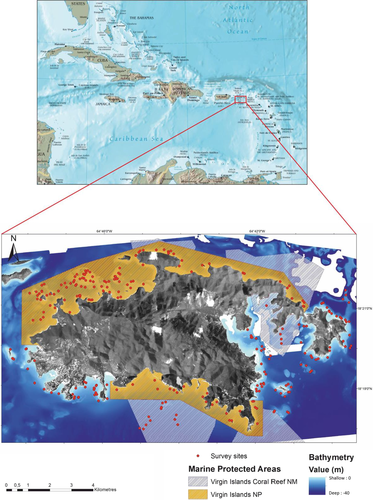
St John is one of three main islands of the USVI located on the Puerto Rican shelf in the Eastern Caribbean (18°20′12.521″N, 64°43′41.1427″W; Figure 1). St John's topography consists of steep slopes, exposed cliffs and dense vegetation. The near-shore seascape of St John supports a complex mosaic of habitat types including seagrass, mangrove and coral reef (including colonized pavement, linear and patch reefs). Coral reefs and associated habitats of the USVI provide important economic, cultural, social and environmental values and benefits to people. The economic value of coral reefs in the USVI has been estimated at $US 187 million annually (Van Beukering, Brander, Van Zanten, Verbrugge, & Lems, 2011). In the past five decades, regardless of protected area designation, coral reef communities in the USVI have declined in structural complexity and ecological integrity owing to a variety of environmental stressors including climate change, disease, coastal development and fishing (Rogers & Beets, 2001). Around St John, live hard coral cover ranges from 0% to 86% (mean 10.41 ± 0.7 [±SE]). Recent comparative analyses on marine protected area performance revealed no significant difference in fish species richness or reef condition inside versus outside of St John MPAs (Pittman, Monaco, et al., 2014; Pittman, Bauer, et al., 2014).
2.2 Data collection
2.2.1 Fish surveys
Survey missions were conducted annually in July from 2002 to 2011 around the island of St John as part of National Oceanic & Atmospheric Administration (NOAA)'s Coral Reef Ecosystem & Assessment Monitoring project (NCREM) operated by NOAA National Centres for Coastal Science (NCCOS) Biogeography Branch in collaboration with the US National Park Service. The number of fish species was quantified from underwater visual surveys of fish at spatially random locations over hardbottom habitat classes as represented in the NOAA benthic habitat map (Kendall et al., 2001). The depth range of samples was 11 ± 0.4 m with a minimum of 0.18 and maximum of 27.6 m.
At each sample location a trained observer on SCUBA swam along a 25-m-long by 4-m-wide belt transect (100 m2 sample unit area) for 15 min maintaining a constant speed while identifying and counting the abundance of all fish observed, including in the water column. The species abundance was recorded in 5-cm size class increments using the visual estimation of fork length (Friedlander et al., 2013). A total of 251 samples from hardbottom habitat within 4 km of the coastline were used in the analysis (Figure 2). Fish data are available online at http://www8.nos.noaa.gov/bpdmWeb/queryMain.aspx.
Taxonomic diversity is a proxy for functional diversity where a greater taxonomic diversity usually represents a greater variety of fundamentally different life histories and functional groups (Warwick & Clarke, 1995). Taxonomic diversity was calculated in the computer software package PRIMER version 6 (Plymouth Routines In Multivariate Ecological Research) from an untransformed species-abundance matrix (Clark & Warwick, 2001). Taxonomic diversity is defined as the average weighted path length between every pair of individuals:
 (1)
(1)where XiXj is the abundance of i and j species and Wij is the distinctness weight given to the path length linking i and j in the hierarchical classification (Clark & Warwick, 2001). Weightings were put on shorter branch lengths in order to have more weight on classes and order than species and genus.
2.3 Within-patch structure
Along each fish transect, fine-scale benthic habitat composition was quantified within 1 m² quadrats at five locations to subsample the 100 m2 fish sample unit area. Estimates of the percentage cover of benthic species and types of biogenic structure such as algae, gorgonians, live coral and sponges were measured in the field by trained scientific divers. From these data additional metrics were calculated to include the coral–macroalgal ratio, maximum hard coral cover, maximum crustose cover and species richness of scleractinian corals. The quadrat locations were pre-selected to ensure a sample was collected at least once within each 5-m length of the transect. The quadrat was divided into 100 (10 × 10 cm) smaller squares to help estimate cover. The percentage of cover was estimated within the quadrat in a 2D plane perpendicular to the observer's line of vision (Friedlander et al., 2013). The topographical complexity (rugosity) was measured using the chain-tape method (McCormick, 1994). Two 6-m-long chains were draped over the substratum along the transect and the distance of the chain along the horizontal tape was recorded by the fish observer. Mean and maximum rugosity were calculated for each survey location.
2.4 Seascape terrain complexity
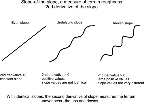
Water depth and the topographical complexity of the sea floor were quantified at multiple spatial scales from a high resolution (3 × 3 m) bathymetric terrain model derived from airborne hydrographic Light Detection and Ranging (LiDAR). The LiDAR sensor measures the difference in the time of reflectance for pulses of high-energy laser to return to the aircraft from the sea floor and the water surface to estimate water depth (Pittman, Costa, & Wedding, 2013). Topographical complexity was measured by applying a slope-of-the-slope morphometric to the digital terrain using a geographical information system (GIS). Slope-of-the-slope, a measure of terrain roughness (Figure 3), was calculated by creating an initial slope surface from the bathymetry and then calculating the slope of the initial slope surface to create a second derivative surface (Pittman, Costa, & Battista, 2009). Slope-of-the-slope has been described as the maximum rate of slope change between neighbouring cells (Pittman et al., 2009).
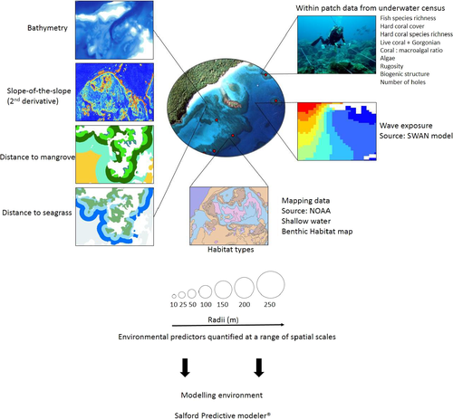
Mean water depth and the maximum slope-of-the-slope were then quantified at multiple spatial scales (seascape sample unit areas of: 10 m radius = 314 m2; 25 m radius = 1,964 m2; 50 m radius = 7854 m2, 100 m radius = 31,416 m2; 150 m radius = 70,686 m2; 200 m radius = 125,664 m2 and 250 m radius = 196,350 m2) surrounding each sample point using a moving window analysis in ArcGIS (ArcGIS Spatial Analyst Neighbourhood Tool; ESRI Inc., http://www.esri.com/).
2.5 Ecological scale selection
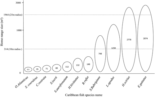
The spatial scale range selected (seascape sample unit area) for quantification of mapped seascape structure was guided by existing data on the known size of fish home ranges for 11 common Caribbean reef associated fishes (mean body length = 14.2 ± 11.7 cm [±SE]). A literature review revealed that home ranges varied widely in size (mean = 752 ± 1098 m²), from 0.5 m² for redlip blenny to 2874 m² for red hind (Table 1). Our analyses were designed to ensure that the scale range selected for the analytical window size overlapped the scale domains for the selected fish home range sizes and extended to encompass the broader surrounding seascape (Figure 4).
| Species name | Home range (m²) | Fork length (cm) | Technique used | Study duration | Location | References |
|---|---|---|---|---|---|---|
| Redlip blenny (Ophioblennius atlanticus) | 0.5 | 5.6 | Visual census and mark-recapture | 1 month | Barbados and Curaçao | Nursall (1977) |
| Juvenile blue parrotfish (Scarus coeruleus) | 35.8 | 4–9.5 | Focal observation | 9 months | Florida Keys | Overholtzer and Motta (1999) |
| Sharpnose puffer (Canthigaster rostrata) | 71 | 5 | Mark and recapture | 1 month | Panama | Sikkel (1990) |
| Striped parrotfish (Scarus iserti) | 80 | NA | Territories marked at regular intervals | 2 months | Belize | Mumby and Wabnitz (2002) |
| Red band parrotfish (Sparisoma aurofrenatum) | 112 | Focal observation | 1 month | Florida Keys | Catano, Gunn, Kelley, and Burkepile (2015) | |
| Caribbean wrasses (Halichoeres bivittatus, Halichoeres garnoti, Halichoeres maculipinna, Halichoeres poeyi, Thalassoma bifasciatum; Labridae) | 132 ± 21.2 | 2–4 | Visual census mark and recapture | 6 months | St Croix, USVI | Jones (2005) |
| Spanish hogfish (Bodianus rufus) | 148 | 22–40 | Visual census | 2 months | Panama | Hoffman (1983) |
| Redfin parrotfish (Sparisoma rubripinne) | 784 | NA | Territories marked at regular intervals | 2 months | Belize | Mumby and Wabnitz (2002) |
| Schoolmaster snapper (Lutjanus apodus) | 1,290 | >24 | Acoustic telemetry | 24 hr | St John, USVI | Hitt, Pittman, and Nemeth (2011) |
| Bluestriped grunt (Haemulon scirius) | 2,778 | >24 | Acoustic telemetry | 24 hr | St John, USVI | Hitt et al. (2011) |
| Red hind grouper (Epinephelus guttatus) | 2,874 | NA | Acoustic telemetry | 152 days | Puerto Rico | Shapiro, Garcia-Moliner, and Sadovy (1994) |
- USVI, US Virgin Islands.
2.6 Seascape patch-mosaic composition & patch proximity
Using techniques from landscape ecology, the seascape mosaic composition (proportion of major patch types) was quantified from a benthic habitat map at multiple spatial extents surrounding each fish sample point. The seascape sample unit was defined using circular buffers (same radii as for terrain metrics) within a GIS for each survey site using the Diversity Calculator tool (ESRI script Diversity Calculator) developed by NOAA Biogeography Branch (http://arcscripts.esri.com/details.asp?dbid=15258).
Patch-mosaic composition was quantified from the NOAA Biogeography Branch Shallow-Water Benthic Habitat map (Zitello et al., 2009), which was mapped with a 100-m-resolution minimum mapping unit. The major cover types of interest were seagrass percentage cover with a map user accuracy of 91.5% (n = 71) and percentage of high complexity hardbottom habitat (a combination of aggregate reef, aggregate patch reef, individual reef, pavement, pavement with sand channels and spur and groove) with a map accuracy of 86.1%. Overall map accuracy for all hardbottom areas was 96% (user's accuracy for hardbottom areas = 97.3%, n = 299; Zitello et al., 2009). In addition to quantifying the area of major habitat types (patch types) we also created a categorical variable of habitat type whereby each individual class of habitat type was assigned a unique value.
To consider the potential effects on fish diversity of connectivity between coral reefs and complementary non-reef habitat types (Olds, Connolly, Pitt, & Maxwell, 2012; Pittman, Caldow, Hile, & Monaco, 2007), we quantified proximity between fish survey sites on coral reefs and the nearest seagrass and mangrove patches. A raster surface of patch proximity was created using Euclidean distance across the insular shelf.
2.7 Wave exposure
Wave exposure can have a considerable influence on the structuring of coral reef fish assemblages (Brown, Harborne, Paris, & Mumby, 2016; Fulton & Bellwood, 2005). Here we quantified the spatial pattern of wave exposure from points predicted across a 240-m-resolution grid using the Caribbean Coastal Ocean Observing System Nearshore Wave Model (Canals-Silander in press) based on the Simulating WAve Nearshore (SWAN) model (Booij, Ris, & Holthuijsen, 1999). The model was designed to be applied in shallow waters with ambient currents, bays, estuaries and channels and provides an annual average of wave power. SWAN is an adaptation of the wave model for deep and intermediate water by incorporation of depth-induced wave breaking and triad wave-wave interactions (Salmon & Holthuijsen, 2015).
2.8 Data analysis
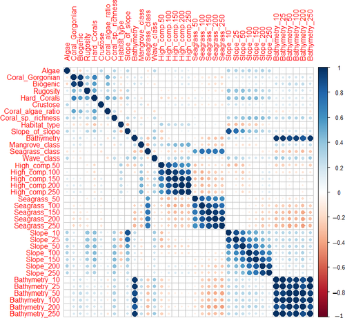
The data for three response variables and 36 explanatory variables were checked for outliers, homogeneity and normality of variance (Table 2). Collinearity amongst predictors and spatial autocorrelation were examined according to the method suggested by Zuur, Ieno, and Elphick (2010).
| Variables | Data source | How it was calculated | Resolution | Mean ± SE (min.–max. values) | |
|---|---|---|---|---|---|
| Unique ID | Survey Index | Transect data | 251 hardbottom surveys sites, with a unique ID and geographical co-ordinates | 100 m² | |
| Response variables | Species richness | Fish visual census. At each sample location a trained observer on SCUBA swam along a 25-m-long by 4-m-wide belt transect for 15 min maintaining a constant speed while identifying and counting the abundance of all fish observed. The species abundance was recorded in 5-cm size class increments using the visual estimation of fork length | 23.6 ± 0.4 (8–44) | ||
| Taxonomic diversity | Calculated in the software PRIMER version 6. Weights were put on shorter branch lengths in order to have more weight on classes and order than species and genus | 58 ± 0.9 (11.6–75.5) | |||
| Richness hotspots | The top 10% of species richness was categorized as 1 and the remaining 90% as 0 | ||||
| Within-patch structures | Live coral + gorgonians | Quadrat data | Sum of the maximum values of live coral and gorgonian cover from the five quadrats on the transect for each location | 100 m² | 10.29 ± 0.5 (0.7–44) |
| Biogenic structure | Sum of sponges, coral and gorgonian cover. The sum of sponges corresponds to the sum of maximum percentage cover of encrusting and upright sponges from the five quadrats | 13.45 ± 0.6 (0.1–48) | |||
| Algae | Sum of maximum percentage cover of turf algae, microalgae, crustose algae and cyanobacteria from the five quadrats | 54.26 ± 1.70–99 | |||
| Live hard coral cover | The maximum values of hard coral and crustose cover, hard coral species richness and coral : macroalgal ratio from the five quadrats on the transect | 10.41 ± 0.7 (0–86) | |||
| Crustose cover | 6.18 ± 0.6 (0–70) | ||||
| Hard coral species richness | 7 ± 0.2 (0–18) | ||||
| Coral: macroalgal ratio | 1.36 ± 0.5 (–1–111) | ||||
| Total maximum holes | Sum of the highest number of small and big holes from the five quadrats | 13 ± 0.8 (0–70) | |||
| Maximum rugosity | Rugosity index measured with the chain tape method, by placing a 6-m chain at two randomly selected start positions ensuring no overlap along 25-m belt transect. The chain was placed such that it follows the relief along centreline of the belt transect. Two divers measured the straight-line horizontal distance covered by the chain | 0.28 ± 0.008 (0.025–0.71) | |||
| Seascape composition | High hard complexity | 2009 NOAA Biogeography Branch Shallow Water Benthic Habitat map | Quantified at a range of spatial scales (10, 50, 100, 150, 200, 250 m radii) using the Diversity Calculator tool in ArcGIS. Detailed geomorphological structures such as aggregate reef, aggregated patch reef, individual patch reef, pavement, pavement with sand channels, spur and groove were considered as having a high hard structural complexity | 100 m | 73 ± 1.5 (0–100) |
| Percentage seagrass cover | The major cover of interest was quantified at a range of spatial scales (10, 50, 100, 150, 200, 250 m radii) using the Diversity Calculator tool in ArcGIS | 2.8 ± 0.5 (0–61) | |||
| Habitat type | 2001 NOAA Biogeography Branch Shallow Water Benthic Habitat map | Ten hardbottom habitats (aggregated reef, aggregate patch reef, individual patch reef, pavement, pavement with sand channels, reef rubble, rock outcrop, sand, sand and scattered coral and rock, spur and groove) | 300 m | ||
| Seascape complexity | Bathymetry mean (10, 50, 100, 150, 200, 250 m radii) | Airborne hydrographic LiDAR (Light Detection and Ranging) | Quantified at a range of spatial scales (10, 50, 100, 150, 200, 250 m radii) using Focal statistics within the Spatial analyst tool | 3 m | 11 ± 0.4 (0.18–27.6) |
| Maximum slope-of-the-slope (10, 50, 100, 150, 200, 250 m radii) | Slope-of-the-slope was calculated by creating a slope surface from the bathymetry and then calculating slope of the initial slope surface. Quantified at a range of spatial scales (10, 50, 100, 150, 200, 250 m radii) using focal statistics within the Spatial analyst tool | 41.75 ± 1 (6.12–82.2) | |||
| Bathymetry classes | The continuous variables were extracted to points using ArcGIS Spatial Analyst tool and then classified into five and seven categories using ArcGIS Reclass tool | ||||
| Slope-of-the-slope classes | |||||
| Wave | Wave exposure | Simulating WAve Nearshore (SWAN)model | Quantified from points predicted using the CariCOOS (Caribbean Coastal Ocean Observing System) | 240 m | 1.12 ± 0.04 (0.1–3.2) |
| Wave exposure classes | The continuous variable was extracted to points using ArcGIS Spatial Analyst tool and then classified into seven categories using ArcGIS Reclass tool | ||||
| Patch proximity | Distance to mangrove and seagrass | Airborne hydrographic LiDAR | To quantify patch proximity between fish survey sites on coral reefs and the nearest seagrass and mangrove patches a raster of patch proximity was created using Euclidean distance across the insular shelf | 3 m |
Mangrove: 1399 ± 69 (63–3826) seagrass: 258 ± 16 (0–1230) |
| Distance to mangrove and seagrass classes | The continuous variable was extracted to points using ArcGIS Spatial Analyst tool and then classified into four and five categories using ArcGIS Reclass tool |
- NOAA, National Oceanic & Atmospheric Administration.
2.8.1 Modelling algorithms
Machine learning algorithms using single classification and regression trees (CART™; Breiman, Friedman, Olshen, & Stone, 1984 1984) and stochastic gradient boosted classification and regression trees (TreeNet™; Friedman & Meulman, 2003) were applied to determine variable interactions and measure variable importance in models of both fish species richness and taxonomic diversity. These non-parametric techniques are more suitable than conventional linear models for exploring complex data that may have multiple structures rather than a single dominant structure (Elith et al., 2006; Hastie, Tibshirani, & Friedman, 2009). Using the same explanatory variable in different parts of the tree, these machine learning algorithms deal effectively with non-linear relationships and higher order interactions that are expected in large complex and multi-scale ecological data sets. Combining CART and TreeNet in exploratory analyses provides high interpretability through the simplicity of CART together with the ability to model higher order interactions using the full suite of variables with TreeNet. In addition, both continuous and categorical data can be incorporated in these models. All models were fitted in the SALFORD PREDICTIVE MODELER® software suite (Salford Systems http://www.salford-systems.com/).
2.9 CART
Fish species richness and taxonomic diversity were analysed as both continuous and categorical variables. The response was transformed into a binary categorical variable with even split (n = 251; high species richness >24 and low species richness <24) and into fish species richness hotspots defined as the top 10 percent of fish species richness (Ceballos & Ehrlich, 2006). CART models were implemented using a standard error rule and a minimum cost tree. The splitting criterion used the Gini index for classification and least squares for regression trees. Trees were generated using a 10-fold cross-validation for testing. The minimum node sample size was set at 3. The optimal tree was the smallest tree with the lowest error. The model starts with the largest tree fitting all the data and then prunes it until it reaches a balance between the smallest numbers of nodes and the smallest error.
2.10 TreeNet™ Stochastic Gradient Boosting
TreeNet (Salford Systems Inc.) is a machine learning algorithm using ensembles of many simple small least squares regression trees or classification trees that are combined through averaging to give improved estimation accuracy (Elith, Leathwick, & Hastie, 2008; Friedman & Meulman, 2003). Boosted regression trees have been demonstrated to outperform many commonly used algorithms (i.e. generalized linear and additive models) for predictive modelling (Elith et al., 2006; Friedman & Meulman, 2003; Pearson, 2015). Boosted trees can model multiple interactions between predictors and are robust to irrelevant predictors and overfitting. Like CART models, trees were generated using 10-fold cross-validation. A very slow learning rate (lr) was set (0.001) and the tree complexity (tc) was six nodes and a maximum of 10,000 trees allowed.
2.11 Variable importance
The relative importance to the optimal model of each variable was estimated from its ranked contribution and the loss of performance when removed from the model. For CART models only, primary splitters were reported here. Surrogates were not taken into account because our data did not have a pattern of missing data. The percentage contribution of each predictor variable was based on the number of times a variable was selected for splitting, weighted by the squared improvement to the model as a result of each split and averaged over all trees (Friedman & Meulman, 2003). The relative contribution of each environmental variable on the response was measured so that the sum adds to 100, with a higher number indicating stronger influence on the response (Elith et al., 2008). Using partial-dependence plots, the effect of a variable on the response after accounting for the average effects of all other variables in the model is represented (Elith et al., 2008). The interactions between predictors were also evaluated using a function testing each possible pair of predictors.
2.12 Model performance
The predictive performance of the final models was evaluated using the co-efficient of determination (R²) for regression analysis and the area-under-the-curve (AUC) of the receiver operating characteristic curve (ROC) for classification trees (Muñoz & Felicísimo, 2004). AUC ranges between 0 and 1 with higher values indicating a better performance. An AUC value of 0.7–0.8 is considered an acceptable prediction; 0.8–0.9 is excellent and >0.9 is outstanding. A value of 0.5 is defined as the predictive ability that could be obtained by chance (Hosmer, Lemeshow, & Sturdivant, 2013).
2.13 Statistical analysis
Data did not meet the assumptions for parametric analysis of variance; therefore, we applied a non-parametric Kruskal–Wallis test to examine differences between categories of variables and spatial scales in their ability to explain the spatial patterns in fish species richness and taxonomic diversity. A multiple pairwise comparison was computed using Dunn's test (Dunn, 1964). Spearman correlations were used to examine the relationship between fish species richness and different categories of variables using the percentage variable importance scores from the predictive models. The mean species richness per mapped habitat type was also investigated to determine differences that may be attributed to the type of habitat rather than its actual physical characteristics. The tests of statistical difference were computed using GRAPHPAD PRISM (version 6.05).
3 RESULTS
3.1 Spatial autocorrelation
Fish species richness data exhibited spatial autocorrelation (Moran's I index: .005, p = .0023) meaning that fish richness were spatially clustered. However, analyses of spatial autocorrelation in the model residuals from CART and TreeNet models were not significant (Moran's I index CART: .01, p > .1, Moran's I index TreeNet: −.008, p > .1), indicating that the model errors were not significantly affected by the spatial autocorrelation in the response data and will not bias co-efficient estimates (Kühn & Dormann, 2012; Figure 5).
3.2 Model performance
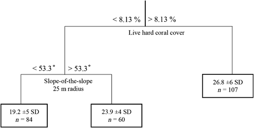
Both CART and TreeNet models showed higher performance when the response variable of fish species richness was classified into richness hotspots (top 10 percent; AUCCART = 0.8, AUCTreeNet = 0.77). Predictive performance of richness hotspots was higher for the CART models than for TreeNet models (overall correct CART = 80.2%; overall correct TreeNet = 71.7%), with low misclassification rates (missclass CART = 6%, missclassTreeNet = 9%). The primary splitters selected by the CART model were live hard coral cover from quadrats, modelled wave exposure and topographical complexity measured by slope-of-the-slope within the 25-m-radius sample unit (1963.5 m²), 50 m (7854 m²) and 150 m (70,686 m²) radius (Figure 6). Models for fish species richness performed better than models for taxonomic diversity (Table 3) and therefore we have focused our results and discussion on the best performing models for fish species richness.
| Responses | Species richness | Taxonomic diversity | Richness hotspots (Top 10%) | |
|---|---|---|---|---|
| Model Performance | R 2 | AUC | ||
| TreeNet | 0.24 | 0.15 | 0.77 | |
| CART | 0.22 | 0.12 | 0.8 | |
| Percentage contribution | ||||
| CART | Live hard coral cover | 100 | 100 | 100 |
| Primary splitters (Figure 5) | Slope-of-the-slope (25m,50m,150m radius) | 50 | 41 | 50 |
3.3 Hypothesis testing
3.3.1 Does within-patch structure explain more of the variability in fish species richness and taxonomic diversity than the surrounding seascape structure?
When comparing the strength of correlations for groups of environmental variables, fish species richness displayed a stronger positive correlation with within-patch variables (Rho = .25, p = .0005) than with patch proximity (Rho = −.02, p = .0139) and seascape composition (Rho = −.03, p = .0002; Figure 7a), but showed a similar strength of association as estimated for seascape terrain complexity Overall, seascape terrain complexity variables yielded a significantly (p = .0006) stronger association with fish species richness than did seascape composition variables.

In addition to a simple correlation co-efficient, the mean percentage contribution of groups of environmental variables as calculated by the TreeNet and CART models was tested to determine if any variable group contributed more than any other (Figure 7b). The between-group contributions to the TreeNet models were significantly (p = .0057) different. Following similar relative patterns as the correlations, pairwise tests revealed that within-patch variables contributed significantly more (p = .0241) to the model than seascape composition variables and wave exposure, therefore highlighting the importance of within-patch variables for predicting fish species richness.
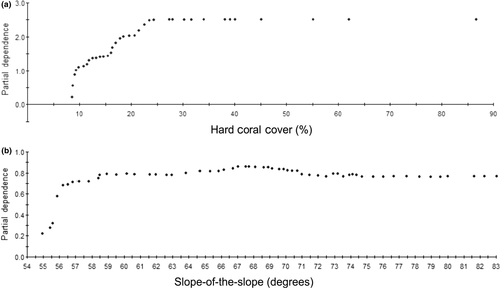
At the level of individual variables, the most important within-patch environmental predictor was live hard coral cover, which displayed a significant (Rho = .45, p = 8.604 E−13) positive correlation with fish species richness. In contrast, a weak negative correlation existed between live hard coral cover and taxonomic diversity (Rho = −.26, p = 2.065 E−5). In fact, taxonomic diversity was more weakly correlated with all environmental variables than species richness. Comparing ranked variable importance scores from both CART and TreeNet models revealed that out of the 41 predictors the most influential single variable for richness hotspots was the amount of live hard coral cover (AUCCART = 0.8, AUCTreeNet = 0.77) followed by slope-of-the-slope at 25, 50 and 150 m radii. In the best CART model, highest fish richness was predicted for coral reefs with coral cover >8.13% and a topographical complexity (slope-of-the-slope) lower than 53.3 degrees. Examination of partial-dependence plots (Figure 8) shows a sharp increase in partial dependence between fish species richness and the amount of live hard coral cover above approximately 8%, tapering off at approximately 25% cover. For slope-of-the-slope, partial dependence with fish species richness increases sharply from 56° to approximately 60°.
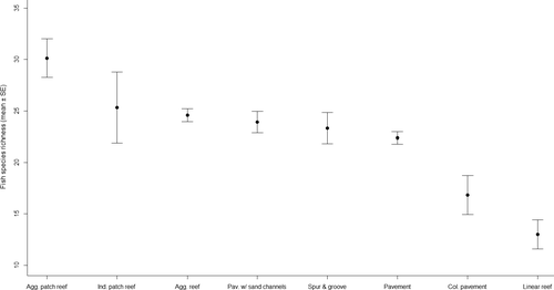
To examine the utility of benthic habitat type as a spatial proxy for fish species richness we grouped fish samples by mapped benthic habitat types and tested for differences, which revealed that mean fish species richness was significantly (p = .0049) different between habitat types. More specifically, mean fish richness was significantly (p = .0034) higher over aggregated patch reef than pavement, colonized pavement and linear reef (Figure 9).
3.3.2 Which spatial scale(s) of seascape patterning best explained fish species richness and taxonomic diversity?
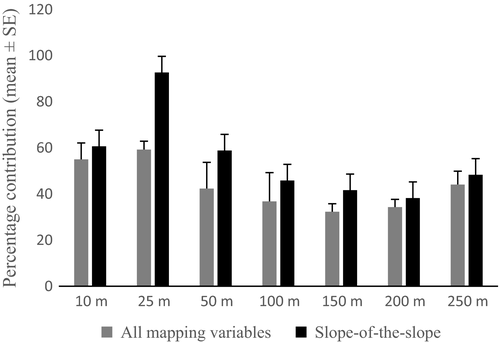
The most influential single spatial scale for seascape patterning was the 25-m-radius seascape equivalent to a sample unit area of 1963.5 m² (Figure 10). The mean contribution to the two models was significantly (p < .05) different between scales. Topographical complexity quantified using slope-of-the-slope within the 25-m-radius seascape sample unit was the most important predictor for fish richness in the TreeNet model (Figure 8) and was a primary splitter in the CART model (Figure 6). The three highest mean percentage contributions were identified with the finer scale seascape sample units of 10–50 m radii.
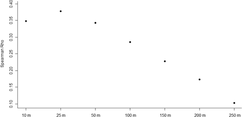
Although fish species richness was most strongly correlated (Rho = .37, p = 6.223 E−10) with slope-of-the-slope at the 25-m-radius scale, this scale of correlation was only statistically higher than the broadest slope-of-the-slope at 250 m radius (Rho = .10, p = .1 ;Figure 11).
3.3.3 Which interacting environmental variables best characterize fish richness hotspots?
The optimal CART model predicted highest fish richness for sites characterized by live hard coral cover >8.13%. Where live hard coral cover was <8.13%, the highest fish richness was found on hardbottom areas where slope-of-the-slope was >53.3 degrees. Lowest fish richness was found on the least topographically complex sites, with lowest live hard coral cover.
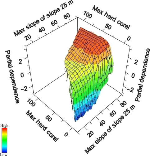
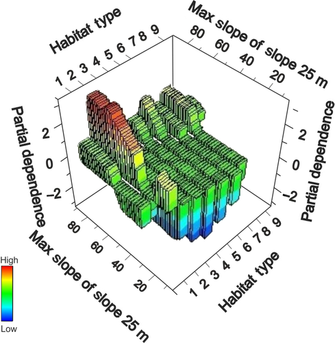
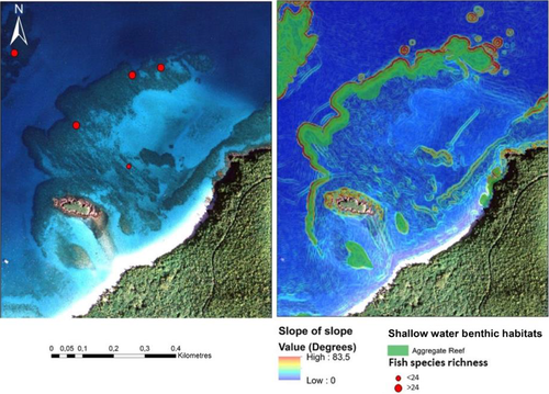
The TreeNet model for fish richness hotspots revealed that interactions between several variables were important in the models (Figures 12 and 13). When examining only the mapping variables, the interaction between slope-of-the-slope at the spatial scale of 25 m and habitat type play an important role in explaining the richness hotspots (Figure 12). The optimal TreeNet model, which allowed multiple interactions between variables, predicted that highest fish richness was found on aggregated patch reefs with highest slope of the slope values (Figure 14).
4 DISCUSSION
Identifying the key environmentaal variables that explain spatial patterns of species richness is an ongoing challenge in ecology and can provide useful information to guide spatial planning and prioritize management actions. Rarely, however, do studies of fish assemblages consider the structure of the seascape surrounding the sampled reef. Our multi-scale seascape ecology approach examined the relative influence of within-patch structural attributes, as well as the surrounding seascape geomorphology, habitat type and area, proximity of complementary habitat types and a key hydrodynamic variable (wave energy) known to influence fish ecology. We found that some of the finest scale measurements (within-patch attributes) explained more of the spatial variation in fish species richness than the surrounding seascape composition (area of habitat types), wave action, and distance to seagrasses and mangroves. However, the best models incorporated interactions between both within-patch and seascape variables, represented by the amount of live scleractinian coral cover measured by SCUBA divers, and the topographical complexity of the sea-floor terrain measured with an airborne laser (LiDAR). The results add additional evidence that the most reliable biophysical characteristics for explaining patterns of fish species richness across coral reefs are the amount of live coral and reef structural complexity (Bell & Galzin, 1984; Coker, Wilson, & Pratchett, 2014; Graham & Nash, 2013; Gratwicke & Speight, 2005; Pittman et al., 2009).
For coral reef conservation, these results highlight the importance of prioritizing actions to focus on enhancing and protecting the amount of live coral and the topographical complexity of reefs, in order to conserve functionally diverse coral reef communities. For future attempts at predictive modelling, our results indicate that higher model performance is likely to be attained by integration of maps of live hard coral cover together with high-resolution bathymetry of the sea floor.
4.1 Model performance
Classification and regression trees modelling provided a clear model in a single small tree, whereas TreeNet models allowed interactions amongst multiple variables in a complex solution combining many hundreds of small trees. Therefore, the simultaneous use of these two algorithms provides the advantage of maintaining the simplicity of interpretation with a CART model, while benefiting from the flexibility provided by ensembles of trees with TreeNet (Fahrnkopf, 2015). The CART model is typically used as an exploratory precursor to the more powerful boosted regression trees, but in this study, it was shown that the predictive performance of the CART model was greater when applied to address the question of predicting richness hotspots (AUCCART = 0.8) than with the continuous variable of species richness (R² CART = .22). With regard to model performance, TreeNet provided no advantage over CART for modelling the binary classification of presence and absence of a richness hotspot (AUCCART = 0.8, AUCTreeNet = 0.77). Not only did the CART model provide good performance in predicting sites with the highest fish richness, it also provided a numerical description of the primary environmental variables that make a coral reef suitable habitat for maintaining high biodiversity. In addition, the breakpoints on the environmental variables that determined the groupings of fish survey sites have potential to help identify thresholds, or ecological tipping points, beyond which species richness abruptly declines or increases (Lintz, McCune, Gray, & McCulloh, 2011).
4.2 Which habitat variables and scales most influence fish diversity?
Our multi-scale analyses demonstrated that within-patch variables (live hard coral cover) and remotely sensed topographical complexity (slope-of-the-slope) contributed to the best models of fish species richness. A high number of fish species (mean species richness 26.8 per 100 m2) was predicted for reefs with live hard coral cover >8.13%. In our study region, approximately 42% of reef sites had at least one quadrat (1 m2) with live hard coral cover >8.13%. This is relatively low when compared with other regions of the Caribbean and reflects a substantial decline since the 1980s (Gardner, Côté, Gill, Grant, & Watkinson, 2003). It has been widely recognized that live hard coral cover has a strong positive correlation with fish species richness (Carpenter, Miclat, Albadalejo, & Corpuz, 1981; Bell & Galzin, 1984) because of coral's provisioning of food, settlement substratum and shelter for a wide range of fishes (Coker et al., 2014; Wilson, Graham, Pratchett, Jones, & Polunin, 2006). In fact, studies on coral reefs have shown that even a very small increase in live hard coral cover (<2%) can result in significant increases in the total number of fish species (Bell & Galzin, 1984). Conversely, however, declines in live hard coral result in declines in fish abundance and species richness (Wilson et al., 2006). Identifying and modelling the link between the amount of live hard coral and the biodiversity of coral reefs is particularly significant because of the documented recent declines in live coral cover owing to a wide range of stressors (Alvarez-Filip et al., 2011). This presents a technical challenge in applied predictive modelling, whereby the difficulty in deriving reliable maps of live coral cover currently hinders efforts to develop spatially continuous predictors for mapping coral-associated biological distributions. Further experimental investigations using remote sensing data are urgently required to identify high spatial resolution data suitable for mapping either directly, or through proxies, fine-scale environmental variables, such as live coral cover and topographical complexity (Hedley et al., 2016; Leiper, Phinn, Roelfsema, Joyce, & Dekker, 2014).
At broader spatial scales (25 m radius) surrounding fish survey sites, topographical complexity measured using slope-of-the-slope (second derivative of bathymetry) served as a good predictor of fish species richness. The utility of spatial metrics of terrain topographical complexity are increasingly being demonstrated through spatial modelling studies for predicting distributions in a wide range of reef organisms and communities from both tropical and temperate environments (Pittman et al., 2009; Pittman & Brown, 2011; Cameron, Lucieer, Barrett, Johnson, & Edgar, 2014; Young & Carr, 2015). Slope and curvature of the sea-floor terrain functions as a proxy for biogenic structural complexity and also influences current flow (Mohn & Beckmann, 2002), which potentially increases food supply for benthic species (Wilson, O'Connell, Brown, Guinan, & Grehan, 2007). Around the island of St John, USVI, reef edges are associated with high topographical complexity (Figure 14), a biogeomorphological pattern that is also associated with high coral cover and fish species richness. The ecological significance of topographical complexity as a key contributor to the geographical distribution of fish richness highlights serious ecological consequences for the long-term capacity of reefs to support high diversity given the recent widespread declines in the topographical complexity of Caribbean reefs (Alvarez-Filip, Dulvy, Gill, Côté, & Watkinson, 2009; Pittman, Costa, Jeffrey, & Caldow, 2010; Rogers, Blanchard, & Mumby, 2014).
In general, seascape predictors played an important contribution only at relatively fine spatial scales across the scale range. For instance, fish species richness was more strongly correlated with slope-of-the-slope at 25-m-radius scale than slope-of-the-slope at 250 m radius. Our review of fish home range areas confirms that the 25-m-radius seascape sample unit encompassed many of the home range areas reported for common Caribbean fish species present in the study area. It is plausible that many of the daily ecological processes for these common species occurred within this space [i.e. the ecological neighbourhood (sensu Cushman & Addicott, 1989)].
However, coral reefs are highly heterogeneous in time and space and not all coral reefs sites surveyed hosted the same amount of fish species even if they did exhibit similar amounts of live hard coral cover and topographical complexity. Fish assemblages comprise very complex interactions amongst physical, chemical and biological processes (Longmore, 2014) that challenge modelling efforts despite including multiple types of environmental variables at multiple spatial scales. Several of our environmental variables made only insignificant contributions to the best models. For instance, patch proximity metrics representing distance from reef to nearest seagrasses and mangroves made a relatively minor contribution to models of fish richness and diversity. This is despite the fact that many species on coral reefs utilize a mosaic of patch types through the life history. Connectivity between coral reefs, seagrasses and mangroves has been shown to influence the structure and function of coral reef fish assemblages where the spatial arrangement of patches and particularly the proximity of patch types influence the strength of interactions (Dorenbosch, Van Riel, Nagelkerken, & Van der Velde, 2004; Mumby, 2006; Mumby, Edwards, et al., 2004; Mumby, Hedley, et al., 2004; Nagelkerken, Sheaves, Baker, & Connolly, 2015; Olds et al., 2012; Pittman, Christensen, Caldow, Menza, & Monaco, 2007). The inclusion of a wide range of reef sites in this study together with assemblages including many species not closely associated with seagrasses and mangroves probably explains the weak influence of proximity. Alternatively, inclusion of patch size attributes together with patch proximity could be examined: i.e. close proximity to large area of seagrass may influence species richness on coral reefs more than equal proximity to only very small patches. Indices that integrate seascape metrics in a functionally meaningful way should be examined in future studies.
Furthermore, classifying highly heterogeneous continuous environmental variables (depth, slope-of-the-slope, wave exposure, distance to patch) into several discrete classes of values to simplify variability did not enhance their contribution to model performance compared with using the original continuous variables. However, we did find that the benthic habitat map classes performed well when allowed to interact with topographical complexity quantified by slope-of-the-slope. Although cost effective and widely available for relatively broad geographical areas, remotely sensed data may not capture sufficient ecological variability to explain the complex patterns of biological distributions for coral reef fishes. Additional types of environmental variables could also be explored such as diver-defined habitat classes, higher resolution terrain models and outputs from connectivity models (Yates, Mellin, Caley, Radford, & Meeuwig, 2016).
4.3 Limitations of the study and future research
Although live hard coral cover exhibited the highest influence on fish species richness and taxonomic diversity, the strength of the bivariate correlation between the amount of live coral and fish response was moderate (Rho fish richness = .45, p = 8.604 E−13) and negatively weak (Rho taxonomic diversity = −.26, p = 2.065 E−5). In addition to the inevitability of missing variables, several other factors related to the fish data collection could result in a weaker than expected association with structural variables, including temporal variability in the fish richness data, which were collected over a period of 10 years. All fish visual censuses took place during daylight hours and therefore we were unable to account for diel cycles and surveys were biased to non-cryptic species. Little is known about the effectiveness of daytime visual surveys as surrogates for multi-phyla diversity patterns, but where destructive sampling has attempted to census the complete fish assemblage on Caribbean coral reefs it is clear that daytime visual census is only reporting on a moderate and visually distinctive proportion of the fishes present (Harborne, Jelks, Smith-Vaniz, & Rocha, 2012; Smith-Vaniz, Jelks, & Rocha, 2006). For example, at Buck Island Reef National Monument in St Croix, USVI, when visual census data and rotenone samples of fishes were compared only 36% of the 228 species sampled with rotenone were detected through visual census (Smith-Vaniz et al., 2006).
One key limitation influencing the application of our models for mapping fish species richness across the study area is that the detailed within-patch variables measured, i.e. live coral cover, are not available as spatially continuous data. Rarely are benthic maps produced that accurately represent the distribution and amount of live coral, although attempts have been made and methods are continually evolving to tackle the challenge (Joyce, Phinn, & Roelfsema, 2013; Mumby, Edwards, et al., 2004; Mumby, Hedley, et al., 2004). However, the results from the study show that live hard coral cover and slope-of-the-slope across spatial scales are positively correlated (Rho = .5, p = 1.87 E−11), suggesting that topographical complexity alone may provide a useful spatial proxy map with which to predict fish species richness as has been demonstrated in Southwestern Puerto Rico (Pittman & Brown, 2011).
At broader spatial extents, questions arise regarding the possible homogenization of the seascape around St John, USVI, and the wider Caribbean. Phase shifts to algal-dominated reefs, declines in structural complexity (i.e. reef flattening) and loss of faunal diversity result in declining structural and functional heterogeneity. Sites will become less different in community composition and diversity, metrics less variable and correlations decoupled. As reefs degrade, it is expected that fish communities will have fewer specialist species and a greater proportion of generalist species (Alvarez-Filip, Paddack, Collen, Robertson, & Côté, 2015). In the last 10 years, fish abundance has declined through the entire Caribbean region (Paddack et al., 2009), particularly large-bodied fishes (Stallings, 2009). Hurricanes, ocean acidification, declining water quality and physical damage from fishing gears are some of the main causes of seascape homogenization causing reef flattening and a general decline in architectural complexity (Alvarez-Filip et al., 2009; Alvarez-Filip et al., 2011). This phenomenon has a negative impact on animal diversity (Seiferling, Proulx, & Wirth, 2014; Smokorowski & Pratt, 2007). Massicotte, Proulx, Cabana, and Rodríguez (2015) found a strong positive relationship between environmental heterogeneity and fish species richness. Further studies should address the ecological consequences of seascape homogenization with a particular focus on the possible alteration of habitat function and the implications for understanding seascape biodiversity patterns.
ACKNOWLEDGEMENTS
We offer our gratitude to the many NOAA data providers including scientific divers and remote sensing analysts at the National Centers for Coastal and Ocean Science Biogeography Branch. We are also grateful to the Marine Institute of Plymouth University for providing research facilities to L. Sekund during a visiting fellowship as part of the International Master of Science in Marine Biodiversity and Conservation. S. Pittman was funded by the NOAA Coral Reef Conservation Program.


