Differential Response of Community Biomass Temporal- and Spatial- Stabilities to Nitrogen Addition in an Alpine Meadow on the Tibetan Plateau
Funding: This work was supported by the National Natural Science Foundation of China (32101267) and the Start-up Funds of Introduced Talent in Lanzhou University (561120205).
Co-ordinating Editor: Francisco I Pugnaire
ABSTRACT
Questions
Community-level stability includes both temporal and spatial dimensions, yet most research has focused on temporal aspects. While considerable progress has been made in understanding community-level temporal stability (α temporal stability), including its interactions with temporal stability at smaller scales (e.g., population or species level) and broader spatial scales (β and γ temporal stability), our understanding of spatial stability at the same community level (α spatial stability or spatial autocorrelation) and its connections to species-level spatial stability and spatial asynchrony remains limited.
Location
An alpine meadow on the Tibetan Plateau, China.
Methods
Using 5 years of data from a nitrogen addition experiment conducted in an alpine meadow on the Tibetan Plateau, we examine the impacts of nitrogen addition on both temporal and spatial stabilities of community biomass, considering species richness, asynchrony, and stability of all species, as well as of dominant and other non-dominant species.
Results
Nitrogen addition influenced the temporal and spatial stability of community biomass by altering the temporal and spatial asynchrony of dominant species and of the overall species level. In this alpine meadow with high species richness, temporal stability of community biomass increased despite a decline in species richness, while spatial stability of community biomass remained unaffected. These results suggest that dominant species dynamics can enhance temporal stability under nutrient enrichment, even as diversity decreases.
Conclusion
Dominant species play a key role in regulating the temporal and spatial stability of community biomass, and the two dimensions of stability respond differently to nitrogen addition. These findings emphasize the importance of incorporating both spatial and temporal facets of stability into ecological theory and ecosystem management under global change.
1 Introduction
The temporal stability of ecosystems, defined as their ability to maintain consistent functioning across years despite environmental variability and disturbances, has received considerable attention from ecologists (Turner et al. 1993; Tilman et al. 2006). In contrast, spatial stability—referring to the consistency or autocorrelation of ecosystem properties among replicate communities under the same treatment within a single year—has received comparatively less attention. This study adopts the term “spatial stability” rather than “spatial autocorrelation” to emphasize its ecological significance in capturing the multidimensional nature of community stability, bridging temporal and spatial perspectives to reveal ecosystem responses to environmental changes. While numerous experimental and theoretical studies have explored temporal stability at various spatial scales (e.g., species temporal stability, alpha temporal stability, beta temporal stability and gamma temporal stability (Hautier et al. 2015, 2020; Wang and Loreau 2016; Wilcox et al. 2017)), the investigation of spatial stability has been relatively limited. Most of these studies have focused on temporal stability across different spatial scales, with fewer addressing the true spatial dimension of stability, which considers fluctuations among replicate plots of the same treatment in the same year (but see Eisenhauer et al. (2011)).
Understanding the mechanisms underlying ecosystem stability in both temporal and spatial dimensions is crucial for predicting the impacts of global environmental changes on ecosystem functioning and sustainability (Donohue et al. 2016; Wang et al. 2019). However, our understanding of the factors influencing spatial stability, distinct from temporal stability, remains limited. While temporal stability has been extensively studied across varying spatial scales (Hautier et al. 2015, 2020; Wang and Loreau 2016; Wilcox et al. 2017), research on spatial stability, defined within the same spatial scales to characterize ecosystem fluctuations among replicate plots of the same treatment in the same year (see definitions below and Figure 1), has been scarce.
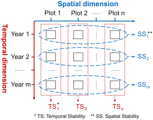
In this context, we define temporal stability (TS) as the mean of aboveground net primary productivity (ANPP) across different years within the same plot (red in Figure 1), divided by its standard deviation along the temporal dimension (Tilman 1999; Lehman and Tilman 2000; Grman et al. 2010). Conversely, spatial stability (SS) refers to the mean of ANPP across different duplicate plots within the same treatment in the same year (blue in Figure 1), divided by its standard deviation along the spatial dimension. Therefore, temporal stability is assessed based on plots as the repetition (e.g., TS1 of plot 1, TS2 of plot 2, and TSn of plot n; Figure 1), while spatial stability is evaluated across parallel years as the repetition (e.g., SS1 of year 1, SS2 of year 2, and SSm of year m; Figure 1). Notably, spatial stability and temporal stability are two dimensions of stability on the same physical scale (e.g., plot scale) and can exist relatively independently. By considering both temporal and spatial dimensions, we can gain a more comprehensive understanding of the mechanisms driving ecosystem stability.
Despite the wealth of research on the effects of nitrogen addition on plant community temporal stability, particularly through changes in species richness (Cottingham et al. 2001; Loreau and De Mazancourt 2013), less attention has been paid to its impact on the spatial dimension of community stability (Hector et al. 1999, 2010; Tilman 1999; Tilman et al. 2006; Cardinale et al. 2012). Experimental evidence suggests that nitrogen addition can reduce community temporal stability by decreasing species richness (Yachi and Loreau 1999; Bai et al. 2004; Loreau and De Mazancourt 2013; Zhang et al. 2017). This reduction in temporal stability may result from the diminished insurance effect, overyielding effect, or portfolio effect brought about by high species richness (Tilman et al. 2006; Hector et al. 2010; Yang et al. 2012; Hautier et al. 2014, 2020).
Conversely, some studies suggest that changes in community temporal stability are primarily driven by shifts in temporal asynchrony and stability among species, independent of changes in species richness (Sasaki et al. 2019; Huang et al. 2020; Valencia et al. 2020; Wu et al. 2020). It is evident that alterations in temporal asynchrony and stability among species, particularly dominant species, play a crucial role in shaping community temporal stability, regardless of changes in species richness (Yang et al. 2011; Xu et al. 2015; Liu et al. 2019). Additionally, the mass ratio hypothesis posits that ecosystem functioning is more influenced by the traits of dominant species than by changes in species richness within a community (Grime 1998; Liu et al. 2019; Rosenfield and Müller 2020). Hence, understanding how ecological factors influence the temporal and spatial stabilities of communities by affecting temporal and spatial stability and asynchrony among species, especially dominant species, is paramount. However, research on these aspects, particularly in the spatial dimension, remains limited.
In this study, we investigate how different levels of nitrogen addition influence community stabilities in both temporal and spatial dimensions through changes in species richness, and asynchrony and stability among species, particularly dominant species. Using a 5-year dataset (2012–2016) from an alpine meadow on the Tibetan Plateau, we address the following questions: (a) How does nitrogen addition affect the stability of community, the asynchrony and stability of species, dominant species, and other non-dominant species in temporal and spatial dimensions? (b) Do the asynchrony and stability of species, especially dominant species, drive the dynamics of temporal and spatial stabilities of communities? (c) Are changes in temporal and spatial stabilities of communities independent of changes in species richness in response to nitrogen additions? Our results highlight significant differences in the responses of temporal and spatial stabilities of communities to nitrogen addition, primarily driven by the varied responses of species, particularly minority dominant species, in temporal and spatial dimensions.
2 Material and Methods
2.1 Study Site
The study was conducted in a relatively flat alpine meadow within the Gannan Grassland Ecosystem National Observation and Research Station (Maqu branch) on the eastern Tibetan Plateau (101°51′44″ E, 33°40′5″ N, altitude 3500 m a.s.l.), Gansu, China. The mean annual temperature is 1.2°C, with monthly temperature ranging from −10°C in January to 11.7°C in July. Precipitation is concentrated in the short, cool summer, with an annual average of approximately 620 mm for the 1975–2012 period. The area receives 2580 h of cloud-free solar radiation annually and experiences over 270 frost days per year (Luo et al. 2006; Zhang et al. 2015). Vegetation in this area is typical alpine meadow dominated by Kobresia spp. (Cyperaceae), Elymus nutans, Agrostis spp., Festuca spp., Poa spp. (Poaceae), Anemone rivularis (Ranunculaceae) and Saussurea spp. (Asteraceae), with an average aboveground dry biomass ranging from 360 to 560 g m−2. Dominant animals include livestock (e.g., yaks, Tibetan sheep, and horses), marmots (Marmota himalayana), zokor (Myospalax spp.), and various ant species.
2.2 Experimental Design
In early May 2011, sixty 10 × 20 m2 plots were established at the study site and enclosed by iron wire fencing. Large herbivores were excluded between March 2011 and October 2011 by fencing, with grazing permitted only during the non-productive winter months. The plots were separated by 1-m buffer strips. Twenty-four plots were designated for a nitrogen (N) addition experiment (Appendix S1), with the remaining plots allocated to experiments involving phosphorus (P) and nitrogen and phosphorus (N & P) addition. This study focused solely on the N addition experiment, which comprised four N addition levels (0, 5, 10, and 15 g N m−2 year−1), each replicated six times. These 24 plots were arranged in a randomized complete block design (Appendix S1). Nitrogen was applied annually as ammonium nitrate (NH4NO3) at the end of May during drizzly conditions to obviate the need for irrigation.
2.3 Species Abundance Measurements
In mid-August of 2012–2016, a 0.5 × 0.5 m2 quadrat was harvested from each replicate of the N addition treatments (24 quadrats per year; 120 quadrats in total). The number of individuals of each species was counted, and the cover of each species and the entire plant community was estimated. For clonal plants, an individual referred to a ramet (Cheplick et al. 1989), equivalent to tillers in graminoids and rosettes or rooting branches in forbs. The fresh aboveground parts (stems, flowers, seeds, and leaves) were clipped, sorted by species, and taken to the laboratory. The fresh parts of each species were dried at 80°C for 48 h and then weighed (0.01 g) to estimate aboveground biomass. Aboveground live biomass served as a measure of primary productivity.
2.4 Statistical Analyses
Biomass was calculated within each plot for the community, four functional groups (sedges, grasses, forbs, and legumes), and dominant and other non-dominant species based on species biomass ranks (Zhang, Kowalchuk, et al. 2019; Zhang et al. 2023). The thresholds for dominant species represented the top 60% of total biomass or more, while other species represented the bottom 40% or less, consistent with previous studies (Clark and Tilman 2008; Soliveres et al. 2016). The proportion of biomass within each plot was calculated for each functional group and the three most dominant species (Elymus nutans, Kobresia capillifolia, and Anemone rivularis), as well as all other non-dominant species, relative to community biomass (Appendix S2). According to our statistical results, the biomass of the three most dominant species (Elymus nutans, Kobresia capillifolia, and Anemone rivularis) under each treatment accounted for 60% or more of the total biomass, while the remaining ones, which include non-dominant species, comprise less than 40% (Appendix S2).
A linear mixed model was fitted using the NLME package in R to examine the effects of nitrogen addition, year, and their interaction on community biomass. In both temporal and spatial dimensions, a series of linear and (where appropriate) quadratic regression analyses were conducted to assess the effect of N addition on the stability and asynchrony for each species set, and the stability of the community. Then, we compared their AIC values and reported the best fit model. Finally, we used piecewise structural equation modeling (SEM) with the ‘piecewiseSEM’ package to evaluate the influence of nitrogen addition on community temporal and spatial stabilities through different pathways (Lefcheck 2016). We conducted hypothetical causal models including all possible pathways in each of temporal and spatial dimensions and improved the model fit by sequentially eliminating non-significant pathways and obtaining simplified models and final models.
For one-way ANOVA, post hoc Tukey's honest significant difference comparisons were employed to compare mean levels within N addition levels. Slope estimates from linear regressions, along with their 95% confidence intervals (CI) and R2 values, were reported to indicate trends in the response of dependent variables to nitrogen addition. Standardized coefficients (r) from SEM were presented to indicate the relative effect of one variable on another in the multivariate partial relationships (Grace et al. 2016). Model fit was assessed using d-separation tests and AIC scores from Fisher's C statistics (Shipley 2013). All analyses were performed using R 3.5.1 (R Core Team 2010).
3 Results
3.1 Spatiotemporal Dynamics of Plant Community in Response to Nitrogen Addition
The linear mixed model indicated significant effects of treatment and year on community biomass (F(1,90) = 16.563, p < 0.001; F(3,20) = 20.036, p < 0.001; respectively; Appendix S7), with no significant treatment × year interactions (F(3,90) = 0.437, p = 0.727; Appendix S7), indicating substantial effects of nitrogen addition on community biomass in both temporal and spatial dimensions (Appendix S7; Appendix S3).
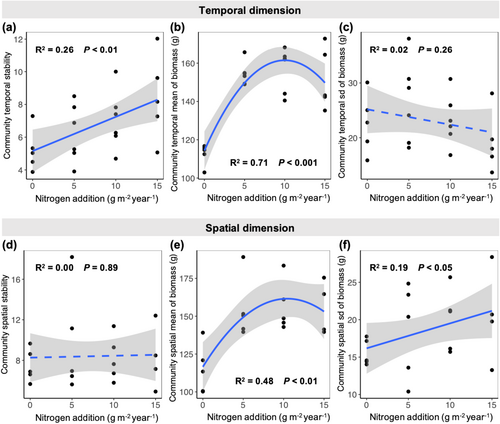
At the community level, nitrogen addition significantly increased the temporal stability of community biomass (R2 = 0.26, p < 0.01; Figure 2a) while leaving the spatial stability of community biomass unchanged (R2 = 0.00, p = 0.89; Figure 2d). According to the changes in the two components (mean and standard deviation (SD)) of the stability calculation formula, this increase in temporal stability was attributed to the significant elevation of the community biomass mean in the temporal dimension (R2 = 0.7, p < 0.001; Figure 2), but non-significant changes in the temporal SD of community biomass (R2 = 0.02, p = 0.26; Figure 2c). On the contrary, the lack of significant change in community spatial stability was attributed to the nitrogen-induced increase in both the mean and SD of community biomass in the spatial dimension (R2 = 0.48, p < 0.01; R2 = 0.19, p < 0.05; Figure 2e,f, respectively).
The three most dominant species, accounting for 60% or more of total biomass (N0: 60%; N5: 68%; N10: 68%; N15: 72%; Appendix S2), exhibited distinct responses to nitrogen addition. Specifically, the percentage of biomass of Elymus nutans increased significantly (N0: 10%; N5: 32%; N10: 37%; N15: 45%; Appendix S2), while the percentage of biomass of Kobresia capillifolia significantly decreased (N0: 41%; N5: 28%; N10: 21%; N15: 18%; Appendix S2), and the percentage of biomass of Anemone rivularis remained relatively stable (N0: 9%; N5: 8%; N10: 10%; N15: 9%; Appendix S2) with nitrogen addition (Appendices S2 and S3).
3.2 Spatiotemporal Dynamics for All Species, Only Dominant Species, and Only Non-Dominant Species in Response to Nitrogen Addition
Considering all species, nitrogen addition significantly increased temporal asynchrony (R2 = 0.32, p < 0.01; Figure 3a) but had no significant effects on spatial asynchrony (R2 = 0.00, p = 0.95; Figure 3e). Additionally, nitrogen addition significantly decreased both temporal and spatial stabilities of species-level biomass (R2 = 0.36, p < 0.01; R2 = 0.15, p < 0.05; Figure 3b,f).
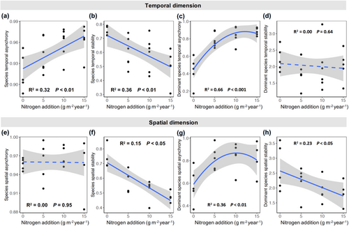
For dominant species, nitrogen addition significantly increased both temporal and spatial asynchronies of biomass of dominant species (R2 = 0.66, p < 0.001; R2 = 0.36, p < 0.01; Figure 3c,g; respectively), while only decreasing spatial stability (R2 = 0.23, p < 0.05; Figure 3h) without affecting temporal stability (R2 = 0.00, p = 0.64; Figure 3d) of biomass of dominant species.
In contrast, nitrogen addition only significantly decreased spatial stability of non-dominant species biomass (R2 = 0.46, p < 0.001; Appendix S4d), with no effect on temporal and spatial asynchronies or temporal stability of non-dominant species biomass (R2 = 0.00, p = 0.61; R2 = 0.10, p = 0.09; R2 = 0.02, p = 0.24; Appendices S4a, S4c, and S4b; respectively).
3.3 Asynchrony of Dominant Species and Its Impact on Temporal and Spatial Stabilities of Community Biomass
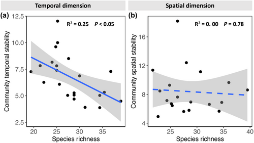
Unexpectedly, temporal stability of community biomass increased significantly with decreasing species richness (R2 = 0.25, p < 0.05; Figure 4a), while spatial stability of community biomass remained unaffected by changes in species richness (R2 = 0.00, p = 0.78; Figure 4b). Structural equation models revealed that the effects of species richness on temporal and spatial stabilities of community biomass were mediated by their impact on temporal and spatial asynchronies of species, particularly dominant species (Appendices S5a and S5b; respectively).
In the temporal dimension, the final model indicated that nitrogen addition's positive effect on temporal stability of community biomass was primarily driven by its direct positive effects on temporal asynchrony of dominant species (r = 0.74, p < 0.001; Figure 5a) and its indirect positive effects on species temporal asynchrony through dominant species temporal asynchrony (r = 0.75, p < 0.001; Figure 5a). Introduction of temporal asynchrony and temporal stability of non-dominant species in the model (Appendix S6a) improved the proportion of variance explained in species temporal asynchrony (from R2 = 0.55 in Figure 5a to R2 = 0.90 in Appendix S6a) and species temporal stability (from R2 = 0.47 in Figure 5a to R2 = 0.90 in Appendix S6a), but did not alter the proportion of variance explained in temporal stability of community biomass (R2 = 0.89 in both Figure 5a and Appendix S6a).
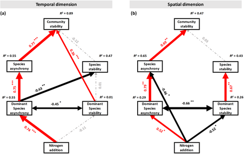
In the spatial dimension, the final model showed that although spatial asynchrony of species positively impacted spatial stability of community (r = 0.69, p < 0.01; Figure 5b), the overall effect of nitrogen addition on species spatial asynchrony was not significant (Figure 3e). This was due to its direct negative effects on spatial asynchrony of species (r = −0.46, p < 0.05; Figure 5b) and indirect positive effects through dominant species (r = 0.52, p < 0.05; r = 0.79, p < 0.01; Figure 5b). Introduction of spatial asynchrony and stability of non-dominant species increased the proportion of variance explained in species spatial asynchrony (from R2 = 0.65 in Figure 5b to R2 = 0.97 in Appendix S6b) and eliminated the direct pathway from nitrogen addition to species spatial asynchrony (r = −0.46, p < 0.05; Figure 5b) without altering the proportion of variance explained in spatial stability of community biomass (R2 = 0.47 in both Figure 5a and Appendix S6a) and species spatial stability (R2 = 0.43 in both Figure 5a and Appendix S6a).
4 Discussion
The findings from our field experiments shed light on the distinct temporal and spatial stabilities of community biomass, which represent two relatively independent dimensions at the α scale. These dimensions, namely α temporal stability and α spatial stability, are different from the temporal stability observed across differing spatial scales (i.e., α temporal stability, β temporal stability, and γ temporal stability). Our results underscore the pivotal role of nitrogen addition in driving the temporal and spatial stabilities of community biomass, primarily through influencing the temporal and spatial dimensions of species asynchrony, particularly among dominant species. Although the presence of asynchrony among non-dominant species enhances the proportion of variance explained in the asynchrony considering all species, its impact on community stability in both temporal and spatial dimensions is relatively minor. Furthermore, the influence of nitrogen addition on the temporal and spatial stabilities of community biomass is partially independent of its effect on species richness. We now delve into the mechanistic underpinnings of these experimental outcomes.
Our delineation of the temporal and spatial dimensions has contributed in three important ways: first, it elucidates the nature of community stability in two distinct dimensions; second, it provided a quantitative method to disentangle these dimensions in field nitrogen addition experiments for the first time; and third, it offers predictive insights into the stability of community biomass in both temporal and spatial dimensions based on the attributes of dominant and non-dominant species. Consistent with previous studies, our results demonstrate that changes in community stability stem from alterations in the mean relative to the standard deviation (SD) of community biomass (Tilman et al. 2006; Hautier et al. 2014; Wang et al. 2019). Specifically, the increased temporal stability of community biomass is attributed to an elevated temporal mean and relatively unchanged temporal SD, whereas the spatial stability remains constant due to concurrent increases in both spatial mean and SD of community biomass. These outcomes align with existing literature, indicating that nitrogen addition typically augments community biomass and its mean (Stevens et al. 2015; Liu et al. 2019; Seabloom et al. 2021), while its effect on SD varies considerably across temporal and spatial dimensions. Consequently, the divergent responses in community stability observed in temporal and spatial dimensions under nitrogen addition can be largely attributed to the similar changes in mean, but the divergent changes in SD of community biomass across these two dimensions.
The observed increase in temporal stability of community biomass in response to nitrogen addition in our study contradicts the findings of most other nitrogen addition experiments, which commonly report a reduction in community temporal stability due to decreased temporal asynchrony among species (Liu et al. 2019; Sasaki et al. 2019; Ma et al. 2021; Wu et al. 2020). Nevertheless, both our results and those of previous studies support the notion that species asynchrony plays a crucial role in driving changes in community stability (Zhang et al. 2016, Zhang, Feng et al. 2019; Huang et al. 2020). In contrast to the findings of other studies, our results demonstrate increased temporal stability and unchanged spatial stability of community biomass under nitrogen addition, primarily attributed to the elevated temporal and unchanged spatial asynchrony of species in this high species richness alpine meadow on the Tibetan Plateau.
In the temporal dimension, increased temporal asynchrony among dominant species positively influences the temporal asynchrony but negatively impacts overall community temporal stability. Conversely, in the spatial dimension, the increased spatial asynchrony of dominant species, coupled with the slight decrease in spatial asynchrony among non-dominant species, collectively results in negligible changes in overall community spatial asynchrony following nitrogen addition. These alterations in overall community asynchrony directly dictate changes in community stability, given the well-established positive effect of species asynchrony on community stability, albeit predominantly in the temporal dimension (Morin et al. 2014; Sasaki et al. 2019; Wu et al. 2020).
The relationship between biodiversity and stability has been a central and enduring topic in ecology, and many theoretical and observational studies have reported a positive correlation between the two (Tilman et al. 2006; Loreau and De Mazancourt 2013; Zhang et al. 2017; Jungers et al. 2021; Wagg et al. 2022). However, our study deviates from this conventional understanding, as we found a negative correlation between species richness and community temporal stability, while species richness appeared to be independent of community spatial stability. Several factors may contribute to this unexpected pattern. First, although alpine meadow communities under ambient conditions typically exhibit high species richness, with 25–45 species per 0.25 m2, our study revealed that the three most dominant species accounted for over 60% of the community biomass, with their overall biomass proportion significantly increasing with nitrogen addition. Second, the dynamics among the three most dominant species, particularly between Elymus nutans and Kobresia capillifolia, were extremely asynchronous in both temporal and spatial dimensions. Finally, the decline in species richness was primarily driven by the loss of rare species, which had a negligible effect on community stability due to their small contribution to community biomass.
Our empirical findings align with the conclusions drawn by Avolio et al. (2014), indicating that shifts in plant community composition, rather than species richness alone, are pivotal drivers of community stability. Notably, the three most dominant species, namely Elymus nutans, Kobresia capillifolia, and Anemone rivularis, representing distinct functional groups (Grasses, Sedges, and Forbs; respectively), collectively constitute over 60% of the community biomass across all treatments and years. Despite exhibiting varied responses to nitrogen addition, these three species consistently maintained their dominance within the community. The asynchronous changes observed among dominant species, spurred by nitrogen addition, led to a transition in the community's dominant functional group from sedges to grasses, alongside an escalation in the asynchrony of all four functional groups across both temporal and spatial dimensions. Specifically, the decline in Kobresia capillifolia biomass (sedge functional group) was offset by an increase in Elymus nutans biomass (grass functional group). These compensatory dynamics among dominant species or functional groups have been proposed as a critical mechanism for enhancing community stability in the temporal dimension (Bai et al. 2004; Connell and Ghedini 2015; Liu et al. 2018; Huang et al. 2020). Our findings underscore the significance of these compensatory effects in bolstering community stability, extending their influence into the spatial dimension.
Several prior studies have underscored the pivotal role of dominant species stability in shaping community stability dynamics (Xu et al. 2015; Ma et al. 2017; Wu et al. 2020). In line with these findings, our structural equation model results revealed that the stability of dominant species directly contributes to community stability in the temporal dimension and indirectly influences community stability by fostering species stability in the spatial dimension. Nevertheless, the impact of dominant species stability on community stability was markedly weaker compared to the influence of dominant species asynchrony across both temporal and spatial dimensions, corroborating findings from previous research (Ma et al. 2017, 2021; Huang et al. 2020). Furthermore, our structural equation modeling demonstrated that the asynchrony of non-dominant species can augment the explanatory power of species asynchrony in both temporal and spatial dimensions, yet its presence did not yield any additional effect on community stability.
In summary, our study sheds light on the dual dimensions of community stability and underscores the critical role of asynchrony among dominant species in upholding community stability across both temporal and spatial dimensions. Importantly, we demonstrate that asynchronous shifts among species, particularly among dominant species in both temporal and spatial dimensions, are essential to safeguard community stability amidst environmental fluctuations and disturbances. These findings underscore the significance of maintaining an ample presence of asynchronous species to uphold the temporal and spatial stabilities of community biomass in the face of global environmental changes.
Author Contributions
P.Z. conceived the research idea; P.Z. and Y.B. performed statistical analyses; P.Z. and Y.B. wrote the paper with contributions from W.W., Z.L., and T.W.; all authors discussed the results and commented on the manuscript.
Acknowledgments
We are grateful to all the people who have helped with our fieldwork. This study was supported by the National Natural Science Foundation of China (32101267) and Start-up Funds of Introduced Talent in Lanzhou University (561120205).
Conflicts of Interest
The authors declare no conflicts of interest.
Open Research
Data Availability Statement
The data are available in https://doi.org/10.6084/m9.figshare.29146658.v1 (Bai 2025).


