Pension Wealth Uncertainty
ABSTRACT
Using a representative sample of Italian investors, we measure the uncertainty of social security benefits by eliciting for each individual the subjective distribution of the replacement rate as a summary indicator of pension uncertainty. We find that pension uncertainty varies across individuals in a way that is consistent with what one would expect a priori, given different information sets and pension schemes. In particular, individuals who are a long way from retirement, and thus face more career uncertainty, report more subjective pension uncertainty. Since expectations reveal information about people's understanding of pension reforms, our findings suggest that they should also be an important determinant of how people respond to reforms.
INTRODUCTION
As a reflection of the still incomplete process of pension reform and of the nature of the reforms adopted, there is a widespread belief that for the citizens of most industrialized countries, pension entitlements have become much more uncertain than in the past. It is fair to say that even an informed worker can find it difficult to estimate her pension benefits at retirement.
The long-term nature of pension arrangements makes it all the more difficult to predict what the eventual pension will be, particularly for younger people. Their longer time horizons mean that young people are more subject to fundamental sources of pension uncertainty, which occur particularly in countries such as Italy, where future benefits will be closely linked to contributions.
The first source of uncertainty is based on the reforms already undertaken, which have resulted in lower public pension coverage, and also, and by design, in greater benefit uncertainty: future pensions will reflect idiosyncratic income uncertainty during a working life, future fluctuations in aggregate GDP growth, and population-wide survival rates. The second source of uncertainty lies in the reforms that have still to be introduced, because the reform process is incomplete. Being unable to predict pension benefits can be of first-order importance to consumer welfare, particularly if perceptions of the true uncertainty are biased, and not sufficient action is taken to buffer against future risk of exhausting lifetime resources. Thus, understanding how much uncertainty people perceive, whether what is perceived is consistent with reality, and how individuals respond to this uncertainty are issues of primary relevance.
In this article, we investigate these issues, focusing on the first two, in the context of the Italian economy. We perform our analysis in three steps. In a first step, we simulate pension benefits according to the Italian pension rules and show that under realistic assumptions pension uncertainty can be summarized by uncertainty about the replacement rate. The simulations show that replacement rate uncertainty is higher for young workers and for workers with more uncertain incomes such as the self-employed. In the new regime in which pensions are tightly linked to contributions, demographic and aggregate income uncertainty are also associated with higher pension uncertainty.
In the second step, we rely on the 2006 Unicredit Customer Survey (UCS), which covers a representative sample of its clients. Since Unicredit is one of the two leading Italian banks and has over 5 million customers, the sample is also representative of the Italian population with a bank account.1 The survey asks for detailed information on income, assets, and demographic variables and, quite uniquely, elicits the subjective probability distribution of the replacement rate (the ratio of the first pension to the final year's income) for each individual in the sample. We rely on subjective distributions to quantify the amount of uncertainty about future pensions that working-age individuals perceive and construct, for each household, the expected replacement rate, and the standard deviation of the replacement rate. Our simple elicitation method of subjective probabilities delivers a high response rate (92 percent of the eligible sample). We find substantial heterogeneity in the expected replacement rate, ranging from 20 percent to the maximum 100 percent, with a sample average of 67 percent. There is also considerable uncertainty about the replacement rate: the sample average of the standard deviation of the subjective replacement rate is 20 percent, with considerable differences across sample participants.
In the final step of our analysis, we show that subjective uncertainty varies across individuals in ways that are consistent with what one should expect a priori, on the basis of observable characteristics (such as age and occupation) and different pension schemes. We find that individuals a long way from retirement, and thus facing more career uncertainty, report more pension uncertainty, and that people with higher income uncertainty are more uncertain also about pension benefits. Income uncertainty is one of the main sources of pension uncertainty in a contribution-based system (such as the one implemented in Italy in 1995). Therefore, our findings reassure us that people are likely to be aware of the uncertainty they face, a necessary condition for them to be able to respond to it.
This is not the first study to measure subjective pension uncertainty. Manski (2004) and Dominitz and Manski (2006) use telephone surveys to measure probabilistic beliefs about pension benefits, while Delavande and Rohwedder (2008) rely on an Internet survey to elicit the subjective probability distributions of pension benefits. Despite the different survey techniques, these studies also find substantial heterogeneity in expected benefits, and large uncertainty. However, unlike our case, they do not relate pension uncertainty to the uncertainty that people should perceive. In addition, our survey provides detailed individual characteristics and measures of income uncertainty.
More generally, our article contributes to a promising avenue of research that embeds questions on preference traits or beliefs in general surveys, such as Scheubel et al. (forthcoming). In the context of pension uncertainty, some recent empirical studies find that subjective pension expectations are related to individual decisions. Liebman and Luttmer (2012) and Delavande and Rohwedder (2011) study the effect of pension uncertainty on, respectively, labor supply, and portfolio choice; Bottazzi et al. (2006) relate subjective point expectations of replacement rates to private wealth accumulation. Our findings that people's expectations contain information about their understanding of pension reforms suggest that these expectations should also be an important determinant of how people respond to reforms. Insofar as these responses are an intended component of the reform (e.g., an increase in private retirement saving), examining people's expectations is one way of assessing a relevant component of the success of the reform.
The article is organized as follows. The “Pension Uncertainty in Italy” section describes the Italian pension system and highlights the sources of uncertainty about future social security benefits. The section “The Subjective Probability Distribution of the Replacement Rate” presents data on individual subjective distributions of replacement rates, and the “Regressions Analysis” section provides evidence on the extent of heterogeneity in respondents' beliefs about pension entitlements. The “Conclusions” section concludes.
PENSION UNCERTAINTY IN ITALY
Until the early 1990s, the Italian social security system featured high replacement rates, earnings-based benefits, indexation of pensions to real earnings and the cost of living, generous provision for early retirement, and a large range of social pensions (i.e., old-age income assistance). As a result, the ratio of pension benefits to GNP reached almost 16 percent in 1992, the highest value among the industrialized countries (Brugiavini, 1999).
The high pension benefits burden on the state budget prompted several reforms, implemented between 1992 and 2008. The main features of these reforms were an increase in the retirement age and the minimum years of contributions for pension eligibility, abolition of seniority pensions for all those who entered the labor market after 1995, and a new formula to compute pension benefits.
As of 2009, workers are classified in three regimes, according to the number of years of pension contribution at end 1995. A defined benefit formula applies to those with 18 years or more of contributions in 1995. We term this formula the “earnings model” and the workers to whom it applies as “old.” Table 1 shows that for this group, pension benefits are proportional to the average of the last 10 years of earnings (15 for the self-employed) before retirement, with an accrual rate of 2 percent for each year of contribution.
| Pension Award Formula | |||
|---|---|---|---|
| Private Sector | Public Sector | Self-Employed | |
| Old | 2% × years of contribution × average of last 10 years of earnings | 2% × years of contribution × average of last 10 years of earnings | 2% × years of contribution × average of last 15 years of earnings |
| Middle-aged | Earnings model before 1995, contribution model after 1995. | ||
| Young | Contributions (33% of gross wage for employees and 20% for self-employed) are capitalized on the basis of the 5-year moving average of GDP growth. The capitalized sum is multiplied by a coefficient that varies by retirement age, taking into account life expectancy. | ||
| Old and Middle-Aged Retiring in | Pension Eligibility Rules | |||
|---|---|---|---|---|
| Seniority Pensions Minimum Years of Contribution | Old Age Pensions Retirement Age | |||
| Private Employees | Public Sector Employees | Self-Employed | ||
| 2008–09 | 35 | 60 | 60 | 61 |
| 2010–13 | 35 | 61 | 61 | 62 |
| After 2014 | 35 | 62 | 62 | 63 |
| Young | 40 | 65 | 65 | 65 |
| (60) | (60) | (60) | ||
- Note: Old, middle-aged, and young refer, respectively, to workers with more than 18 years of contributions in 1995, less than 18 years of contributions in 1995, and those who started working after 1995. Figures in parentheses are retirement ages for women.
 (1)
(1)In Equation (1), Y denotes earnings, N retirement age, τ the contribution rate, g a 5-year moving average of the GDP growth rate, and γ the annuitization factor. The contribution rate is 33 percent for private and public sector employees. One-third of the contribution is paid by the employee, and two-thirds by the employer. Historically, the self-employed have a different contribution regime. The contribution rate is 20 percent of yearly income, roughly two-thirds of the contribution paid by employers for public and private sector employees. As a consequence, the self-employed are entitled to substantially lower pensions than private and public sector employees.
The third group of workers includes all those with at least 1 year but less than 18 years of contributions in 1995 (“middle-aged”). For this group, benefits are a weighted average of the benefits computed according to the earnings and contributions models, with weights given by the proportion of the working career under the two regimes (before and after 1995). This shows that there is considerable heterogeneity of pension benefits: more generous provisions for those near retirement, and lower benefits for self-employed relative to private and public sector employees, regardless of pension regime.
The lower panel in Table 1 shows that pension eligibility also varies substantially. For the old and middle-aged, the retirement age is 60 years (61 for self-employed), with a minimum of 35 years of contributions. The retirement age will increase gradually up to 2014, to 62 years for private and public sector employees and 63 years for self-employed. The young will be eligible to retire after 40 years of contributions or after age 65 (60 for females).
In this article, we focus on the replacement rate, defined as the ratio of the first pension payment to the last preretirement income payment, as a synthetic indicator of pension wealth. While we recognize that pension wealth also depends on retirement age, which possibly is uncertain, we argue that retirement age uncertainty is less important than replacement rate uncertainty, partly because individuals can control more directly for retirement age within a relatively narrow window set by the law, and partly because individuals tend to retire at the minimum statutory age. To verify this claim, we exploit our data, which also record subjective expectations on retirement age.
Even without any possible changes to legislation in the future, forecasting one's pension is not an easy task because future benefits depend on occupation (self-employed vs. private and public sector employees), earnings profile, and earnings volatility. For the young, future pension benefits depend also on demographic shocks (reflected in the annuitization factor γ) and GDP growth.
To link pension uncertainty to individual income uncertainty, aggregate income uncertainty, and demographic uncertainty, we perform simple simulations of the pension benefits in different scenarios.3 Our simulations make two important simplifying assumptions. First, while we allow for uncertainty in the underlying factors (γ, g, and w, annuitization factor, income, and GDP growth, respectively), we assume that the pension award formula (1) will not change in the future. Second, we assume that pension uncertainty does not affect labor supply, and therefore retirement decisions.

In the baseline calculations, we assume that the average GDP growth rate is 1.5 percent per year (in line with the average growth rate of the Italian economy in the last two decades), the annuitization factor γ is 0.0551 (under the current rules, this is the annuitization factor for those retiring at age 62), and the standard deviation of transitory and permanent income shocks is 1 percent (see footnote 4). Under these assumptions, the expected replacement rate is 61.7 percent for an employee (τ = 0.33) and 37.4 percent for a self-employed person (τ = 0.20).
Figure 1 plots the coefficients of variation of the replacement rate distribution against age in the contribution model (those who entered the labor market after 1995). Pension uncertainty is about four times higher for someone just entering the labor market (at age 25) than for someone retiring after 37 years at age 62. The reason is that income uncertainty is much larger for a young person than for someone close to retirement. Doubling the standard deviation of permanent income shocks (σv = 0.02) also doubles pension uncertainty (see dashed line in Figure 1).4
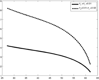
Note: The simulations assume that the growth rates of individual annual earnings and aggregate GDP are, respectively, 2 percent and 1.5 percent; the retirement age is 62; the number of years of contributions is 37; the annuitization factor is 0.0551; and the mean of transitory and permanent income shocks is 1. The continuous line is obtained by setting the standard deviations of permanent (σv) and transitory (σu) income shocks to 1 percent, and the dashed line by setting σu to 0.01 and σv to 0.02.
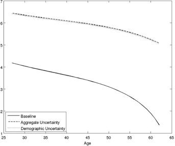
Note: The simulations assume that the growth rate of annual earnings is 2 percent, the retirement age is 62, the number of years of contributions is 37, the mean of transitory and permanent income shocks is 1, and σu = σv = 0.01. The continuous line is obtained by setting the annuitization factor to 0.0551 and the GDP growth rate to 1.5 percent; the dashed line assumes that GDP growth is uniformly distributed between 1 and 2 percent, and the annuitization factor is 0.0551; and the dotted line is obtained assuming that the annuitization factor is uniformly distributed between 5 and 6 percent and the GDP growth rate is 1.5 percent.
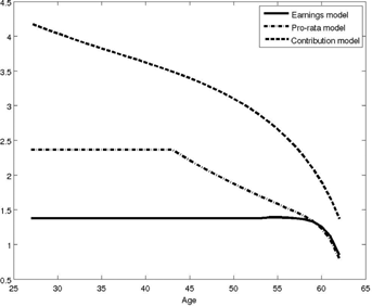
Note: The simulations assume that the growth rate of earnings and aggregate GDP are respectively 2 and 1.5 percent per year, the retirement age is 62, the number of years of contributions is 37, the annuitization factor is 0.0551, the mean of transitory and permanent income shocks is 1, and σu = σv = 0.01. In the pro rata regime the year of job market entry is 1977. The continuous line refers to the earnings model, the dot-dash line to the prorata regime, and the dashed line to the contribution model.
Uncertainty about future GDP growth (as reflected in the g factor) and demographic developments (as reflected in γ) are two further sources of pension uncertainty. Their effects are documented in Figure 2: the continuous line refers to the baseline case, the dashed line assumes that the growth rate of GDP is uncertain and uniformly distributed between 1 and 2 percent, and the dotted line assumes that the annuitization factor is uncertain and uniformly distributed between 5 and 6 percent. Figure 2 shows that pension uncertainty increases by about 3 percentage points at each age when aggregate GDP growth is uncertain; the effect of demographic uncertainty is quantitatively similar.
Pension uncertainty varies also across different pension regimes. Figure 3 compares regimes for a private employee. In the earnings model for the old, pensions are proportional to the last 10 years of earnings, and pension uncertainty is considerably lower: the coefficient of variation is 1.4 percent until age 52 (10 years before retirement) and then falls gradually to less than 1 percent just before retirement. Not surprisingly, in the regime for middle-aged, the coefficient of variation ranges between the earnings and the contribution models.
To summarize, our simple simulations show that pension uncertainty is higher for young workers and workers with more uncertain incomes such as self-employed. Furthermore, in the new contribution-based regime, demographic and aggregate income unpredictability increases pension uncertainty. To check whether people actually perceive the pension uncertainty implied by current legislation, in the section “The Subjective Probability Distribution of the Replacement Rate,” we use subjective expectations of replacement rates to construct individual replacement rate distributions. It should be noted that the degree of uncertainty produced by our simulation depends on the particular parameters of the model. Thus, we cannot compare directly the level of subjective and simulated pension uncertainty. However, we can check whether observable differences in subjective pension uncertainty are consistent with the simulations discussed above.
THE SUBJECTIVE PROBABILITY DISTRIBUTION OF THE REPLACEMENT RATE
Several surveys attempt to measure subjective expectations of Social Security benefits. In the United States, Bernheim (1988) analyzes the accuracy of preretirement expectations concerning social security benefits in the Retirement History Survey, and Gustman and Steinmeier (1989, 2005) study point expectations of the level of future benefits available from the Health and Retirement Study.
Dominitz and Manski (2006) go a step further. Using the Survey of Economic Expectations (SEE), they study the probabilistic expectations of social security retirement benefits. SEE is a telephone survey addressed to individuals aged 18–69, who are asked first to report the lowest possible and highest possible levels of their future benefits. Their responses are used to set thresholds for up to six probabilistic questions about the level of their benefits. The subjective probabilities elicited from respondents are used to fit a respondent-specific parametric distribution following the procedure described in Manski (2004).5
Delavande and Rohwedder (2008) measure future pension benefits via an Internet survey of respondents to the Health and Retirement Study, which is representative of the U.S. population aged 51 and over. They obtained a distribution of pension benefits using the Dominitz and Manski percent chance format and a visual representation of future benefits.6 Both formats generate a similar central tendency, but the percent chance format generates a more widely dispersed distribution. Furthermore, the dispersion of the elicited distribution is correlated to other sources of uncertainty (such as years to expected claiming age and subjective probability of losing one's job in the next year), in the expected direction for both designs. Overall, Delavande and Rohwedder's findings suggest that the main advantage of the visual over the percent chance format is that it minimizes the loss of observations due to inconsistencies.7
Disney and Tanner (1999) and Bottazzi et al. (2006) analyze point expectations of the replacement rate for the United Kingdom and Italy, respectively. In line with these studies, we focus on replacement rate distribution uncertainty rather than uncertainty in the level of future benefits. The two are not directly comparable. Some workers might be uncertain about their future level of benefits, but much less uncertain about their replacement rate. For example, consider a situation in which benefits are proportional to income received in the last year of paid work (as was the case for Italian public employees before the 1995 reform). Since income in the last year is uncertain, she might be uncertain about the level of benefit, although she knows the replacement rate with certainty. On the other hand, an uncertain replacement rate signals an uncertain pension benefit except in the extreme case in which the replacement rate is perfectly negatively correlated with the final year's income.
In this article, we use subjective expectations available in the 2006 Unicredit Survey (UCS), a representative sample of Unicredit customers. The interviews were conducted between May and September 2007 by a leading poll agency using Computer Assisted Personal Interviews. The total sample size is 1,686 customers; the replacement rate questions were addressed to 1,024 working individuals (employees and self-employed). The section titled “The Survey” in the Appendix includes further details on the survey, and compares sample statistics with the 2006 SHIW. In particular, it explains that the sample design is similar to that used by the Bank of Italy SHIW. The two samples have similar characteristics. As shown in Table A1 in the Appendix, compared to Italian households surveyed in the 2006 SHIW, the Unicredit sample is slightly older, more educated, less likely to work in the manufacturing sector, and more likely to live in the North of Italy. However, when we compare the UCS with SHIW respondents with a bank account, we find that the samples are quite similar in terms of demographic characteristics (age, gender, education).
Elicitation Method
To elicit pension expectations in the UCS, we follow a procedure similar to Dominitz and Manski (2006). All employees and self-employed (1,024 observations) were asked first to report the minimum (ym) and maximum (yM) values of the replacement rate and then, on a 0–100 scale, to rank the probability that the replacement rate will be lower than the mid-point between the minimum and the maximum, Prob(y ≤ (ym+ yM)/2) = π. The question was worded as follows:
- (1) At the time of retirement, what is the minimum fraction of labor income that you expect to receive? (ym)
- (2) And what is the maximum value? (yM)
- (3) What is the chance that the fraction will be greater than X (where X is computed by the interviewer as (ym + yM)/2? In other words, if you were to assign a score between 0 and 100 to the chance that the fraction will be greater than X, what score would you assign? (“0” if you are certain to receive a pension greater than X, “100” if you are certain to receive a pension less than X). The following table was shown to the respondent:

To estimate the moments of the subjective distributions of the replacement rate we rely on the assumptions and methods first applied by Guiso et al. (2002) for the subjective distribution of future income. We assume that the subjective distribution is either uniform or triangular, and based on the elicited values of ym, yM, and π, we compute the respondent-specific mean, standard deviation, and coefficient of variation. The formulae of these statistics are reported in the section titled “The Subjective Probability Distribution of the Replacement Rate” in the Appendix.8
We set to missing values observations where ym, yM, or π are missing and all cases where respondents provide inconsistent answers (ym ≥ yM). The resulting sample includes 92 percent of the original sample (940 observations).9 The fraction of nonmissing values is much higher than the 66 percent value in Dominitz and Manski (2006), but somewhat lower than the 97 percent of usable answers in Delavande and Rohwedder (2008).10
Descriptive Statistics
The top panel in Table 2 reports cross-sectional statistics of the central tendency and dispersion of the subjective replacement rate distribution. The median expected replacement rate for the sample of 940 valid observations is 71 percent (for both the uniform and triangular distributions), close to the statutory rate for an average individual in the sample (median 70 percent).11 Although there is substantial heterogeneity in expected replacement rates, on average, expectations parallel the legislation. The dispersion of the subjective replacement rate depends on the assumptions made about the distribution. Assuming that the distribution is uniform, the median of the respondent-specific coefficient of variation is 3.4 percent (2.4 percent using the triangular distribution). The average coefficients of variation are slightly higher (4.34 percent and 3.11 percent, respectively). The data also allow estimation of the subjective distribution of retirement age. Interviewees were asked to provide minimum and maximum values for the expected retirement age, and to indicate the probability that this age would be greater than the mid-point of the range. We apply the same procedure used for replacement rates to estimate the respondent-specific subjective distributions of retirement age. The cross-sectional statistics of the central tendency and dispersion of that distribution are reported in the bottom panel of Table 2. The median is just below 64 for both the uniform and the triangular distributions, in line with current legislation. Retirement age uncertainty, while not negligible, is lower than replacement rate uncertainty: on average, the coefficient of variation is 1.47 percent using the uniform distribution (1.06 percent using the triangular). Since the pension award formula suggests that replacement rates depend—among other factors—*also on retirement age, replacement rate uncertainty should reflect also retirement age uncertainty.12 Therefore, in the rest of the section, we focus on the replacement rate as the main driver of pension uncertainty.
| Statistics of the Subjective Distributions | Cross-Sectional Statistics | ||||
|---|---|---|---|---|---|
| Mean | Median | Standard deviation | Minimum | Maximum | |
| Replacement rate mean | |||||
| Uniform | 67.15 | 71.13 | 19.54 | 1.00 | 100.00 |
| Triangular | 67.24 | 71.33 | 19.48 | 1.00 | 100.00 |
| Standard deviation | |||||
| Uniform | 2.48 | 2.47 | 2.24 | 0.00 | 17.06 |
| Triangular | 1.78 | 1.78 | 1.59 | 0.00 | 12.08 |
| Coefficient of variation | |||||
| Uniform | 4.34 | 3.40 | 4.56 | 0.00 | 40.62 |
| Triangular | 3.11 | 2.41 | 3.22 | 0.00 | 28.10 |
| Retirement age mean | |||||
| Uniform | 64.37 | 63.75 | 5.88 | 21.05 | 100.00 |
| Triangular | 64.36 | 63.68 | 5.85 | 21.20 | 100.00 |
| Standard deviation | |||||
| Uniform | 0.95 | 0.85 | 0.92 | 0.00 | 11.37 |
| Triangular | 0.68 | 0.60 | 0.65 | 0.00 | 8.06 |
| Coefficient of variation | |||||
| Uniform | 1.47 | 1.34 | 1.39 | 0.00 | 15.80 |
| Triangular | 1.06 | 0.96 | 0.99 | 0.00 | 11.29 |
- Note: The table reports cross-sectional statistics computed from the moments of the subjective replacement rate and retirement age distributions. The number of observations is 940.
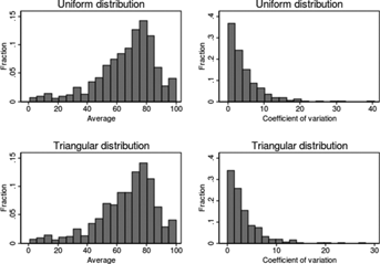
While cross-sectional averages are useful to describe the subjective distribution of the average individual, they hide important sample heterogeneity. Figure 4 plots the cross-sectional distribution of the mean and coefficient of variation of the 940 respondent-specific distributions. The figure highlights considerable heterogeneity in the responses. For instance, 10 percent of respondents expect a replacement rate of less than 40 percent, while another 10 percent expect it to be over 85 percent. The proportion of respondents that report minimum expected replacement rate equal to the maximum (therefore expressing no uncertainty) is 25 percent.13 On the other hand, for 9.6 percent of the sample the coefficient of variation exceeds 10 percent. The next step in the analysis is to relate pension expectations to individual characteristics. Given the features of the current pension regimes, we are particularly interested in studying how the subjective probabilities correlate with individual characteristics (such as age and occupation) that should influence pension uncertainty.
REGRESSIONS ANALYSIS
The elicited expectations quantify the extent of heterogeneity in individuals' beliefs and help to assess how individual characteristics are related to the subjective probabilities. Figure 5 presents kernel-smoothed means of the average and coefficient of variation of the respondent-specific replacement rate distributions, by education and age. In Figure 5 and in the rest of the article, we focus on the triangular distributions (by construction, the uniform distribution is more dispersed, but results are qualitatively similar). The graphs in Figure 5 show that the expected replacement rate increases with age (upper left panel) but is not strongly correlated with education (bottom left panel). In particular, 35-year-old workers expect a replacement rate of 63 percent, while workers close to retirement expect a replacement rate of 70 percent or higher. As explained in the “Pension Uncertainty in Italy” section, a positive relation between age and expected replacement rate mirrors the features of current pension legislation, which grants more generous pensions to workers close to retirement.
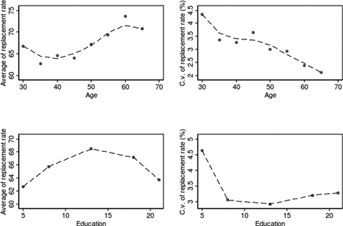
The dispersion of the replacement rate distribution declines substantially during the life cycle, signaling that younger workers perceive substantially more uncertainty than workers close to retirement. In the upper-right panel, the coefficient of variation is 4.5 percent for 30-year-olds and about 3 percent for workers over 60. The lower-right panel shows that workers with lower levels of education face substantially higher pension uncertainty than workers with high school or college degrees, reflecting the higher earnings volatility of blue-collar jobs.
To investigate these relations in more depth, Figure 6 presents kernel-smoothed 0.25-, 0.50-, and 0.75-quantile regressions of the subjective central tendency and dispersion of the subjective distributions by age and education groups. Figure 6 shows that pension uncertainty is substantially higher among young persons at each quantile (upper-right panel), confirming the evidence in Dominitz and Manski (2006). Even middle-aged workers tend to be rather uncertain about their future pension entitlements. The negative relation between uncertainty and age is in line with the simulations in the “Pension Uncertainty in Italy” section.
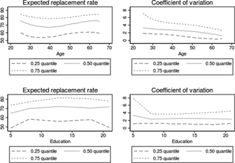
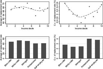
Figure 7 plots the means and coefficient of variation of the respondent-specific distributions by occupation and income deciles. It shows that expected replacement rates do not vary with income (upper-left panel), while the relation between income and the coefficient of variation is nonlinear (upper-right panel): uncertainty is greatest at the lowest and highest ends of the income distribution. Furthermore, professionals and self-employed, who will receive lower pensions because of their lower contribution rates, do indeed expect their pensions to be lower (lower-left panel). They also perceive greater pension uncertainty; given the pension award formula, this is in line with the fact that they also face higher income volatility, as shown by the simulations in Figure 3.
The final step is regression analysis to summarize the correlations between subjective expectations and individual characteristics. Table 3 presents OLS regressions of the measures of the mean, standard deviation, and coefficient of variation of the respondent-specific distributions of the replacement rate. The independent variables include demographic variables (age, gender, education), sector dummies (agriculture, industry, public sector), occupation dummies (professionals, self-employed), region of residence, and dummies for income quartiles.
| Expected Replacement Rate | Standard Deviation | Coefficient of Variation | ||||
|---|---|---|---|---|---|---|
| (1) | (2) | (3) | (4) | (5) | (6) | |
| Male | –1.320 | –1.239 | 0.185 | 0.166 | 0.179 | 0.158 |
| (1.434) | (1.436) | (0.122) | (0.122) | (0.243) | (0.244) | |
| Age | 0.270 | 0.271 | –0.017 | –0.017 | –0.038 | –0.038 |
| (0.059)*** | (0.059)*** | (0.005)*** | (0.005)*** | (0.010)*** | (0.010)*** | |
| Education | 0.039 | 0.054 | –0.002 | –0.005 | –0.009 | –0.013 |
| (0.192) | (0.193) | (0.016) | (0.016) | (0.033) | (0.033) | |
| Agriculture | –2.257 | –2.367 | –0.130 | –0.105 | 0.103 | 0.130 |
| (3.700) | (3.702) | (0.315) | (0.314) | (0.628) | (0.628) | |
| Public sector | 4.133 | 4.147 | –0.290 | –0.293 | –0.750 | –0.754 |
| (1.597)*** | (1.597)*** | (0.136)** | (0.135)** | (0.271)*** | (0.271)*** | |
| Industry | 2.228 | 2.173 | –0.249 | –0.236 | –0.419 | –0.406 |
| (1.619) | (1.620) | (0.138)* | (0.137)* | (0.275) | (0.275) | |
| Professional | –11.261 | –11.275 | 0.420 | 0.423 | 1.482 | 1.486 |
| (1.722)*** | (1.722)*** | (0.146)*** | (0.146)*** | (0.292)*** | (0.292)*** | |
| Self-employed | –8.764 | –8.793 | 0.302 | 0.308 | 1.082 | 1.090 |
| (1.609)*** | (1.609)*** | (0.137)** | (0.136)** | (0.273)*** | (0.273)*** | |
| Northeast | –1.853 | –1.875 | –0.202 | –0.197 | –0.301 | –0.296 |
| (1.887) | (1.887) | (0.160) | (0.160) | (0.320) | (0.320) | |
| Center | 5.165 | 5.059 | 0.163 | 0.188 | –0.024 | 0.002 |
| (1.840)*** | (1.843)*** | (0.156) | (0.156) | (0.312) | (0.313) | |
| South | 6.375 | 6.309 | –0.044 | –0.029 | –0.555 | –0.539 |
| (1.836)*** | (1.837)*** | (0.156) | (0.156) | (0.312)* | (0.312)* | |
| Small city | 0.920 | 0.927 | 0.256 | 0.254 | 0.064 | 0.062 |
| (1.753) | (1.753) | (0.149)* | (0.148)* | (0.298) | (0.297) | |
| II income quartile | 0.756 | 0.770 | –0.443 | –0.446 | –0.646 | –0.650 |
| (1.795) | (1.795) | (0.153)*** | (0.152)*** | (0.305)** | (0.305)** | |
| III income quartile | –0.236 | –0.222 | –0.353 | –0.356 | –0.444 | –0.448 |
| (1.787) | (1.787) | (0.152)** | (0.151)** | (0.303) | (0.303) | |
| IV income quartile | –0.632 | –0.498 | –0.188 | –0.219 | –0.177 | –0.211 |
| (1.876) | (1.880) | (0.159) | (0.159) | (0.318) | (0.319) | |
| Index of financial | –0.437 | 0.102 | 0.110 | |||
| literacy | (0.426) | (0.036)*** | (0.072) | |||
| Constant | 54.470 | 55.695 | 2.710 | 2.425 | 5.275 | 4.968 |
| (4.378)*** | (4.538)*** | (0.372)*** | (0.384)*** | (0.743)*** | (0.770)*** | |
| Observations | 940 | 940 | 940 | 940 | 940 | 940 |
| R2 | 0.13 | 0.13 | 0.06 | 0.07 | 0.09 | 0.09 |
- Note: The table reports OLS estimates. Standard errors are reported in parentheses. *** indicates statistical significance at the 1 percent confidence level, and statistical significance at the 5 percent level, and *statistical significance at the 10 percent level. The omitted categories are: services, private employees, Northwest, and income quartile dummies.
The estimates in Table 3, column (1) confirm that older workers expect a higher replacement rate than younger ones, owing to the more generous pension award formula (linked to average earnings in the 10 or 15 years before retirement rather than to contributions over the entire career).14
Public sector employees replacement rate expectation that is 4.1 percent higher than that of private employees (the omitted category), while professionals and self-employed expect a replacement rate 11.3 and 8.8 points lower, respectively. Residents in Central Italy expect a replacement rate that is 5.2 points higher than individuals living in the North West (the omitted category), while residents in the South expect a 6.4 point higher replacement rate. These effects are likely to reflect regional heterogeneity in the occupation and income distribution.
The ability to process financial information and perceive uncertainty depends on formal education (as measured by years of schooling) but also on financial literacy. In column (2) of Table 3, we add to the set of controls an index of financial literacy computed from survey responses. We compute the index defining two dummy variables equal to 1 if respondents answer questions on interest rates and inflation correctly,15 four dummies that measure the ability to rank asset risk correctly,16 and two dummies related to the ability to understand the concept of financial diversification and to rank the risk of specific portfolios.17 The index of financial literacy ranges from 0 (no questions answered correctly) to 8 (all correct answers), with a median of 3. Column (3) shows that people with above average financial literacy tend to expect a lower replacement rate. However, the coefficient is not statistically different from zero.18
In Table 3, columns (3) and (4) the dependent variable is the standard deviation of the respondent-specific subjective distribution of the replacement rate.19 Pension benefits are more uncertain for professionals and self-employed than for employees, consistent with their greater income volatility and different pension regime. Perceived pension uncertainty falls with age, in line with the descriptive analysis and the findings in Dominitz and Manski (2006). The age coefficient captures several effects: first, and most important, lifetime income uncertainty is higher for younger workers; second, pension regimes differ according to age—earnings related for older workers and contribution based for younger ones; third, in the contributions regime, benefits depend on a broader range of variables, including GDP growth expectations and demographic uncertainty, which are likely to vary with age. Moreover, as discussed in the “Pension Uncertainty in Italy”, section, the contribution method potentially amplifies the effect of income uncertainty on pension uncertainty. Finally, individuals presumably have a stronger incentive to learn about benefits as they are near retirement, reducing perceived uncertainty. Unfortunately, the data do not contain enough information to distinguish between these different explanations.
The standard deviation of the replacement rate distribution is positively associated with the index of financial literacy: an increase in the index of 1 is associated with a 0.2 point increase in the standard deviation, and around 6 percent increase in the sample mean. This suggests that better financially informed investors may also be more aware that pensions are uncertain.20
For robustness, in Table 3, columns (5) and (6) we report regressions where the dependent variable is the coefficient of variation of the replacement rate distribution. The results confirm that perceived pension uncertainty is greater for professionals and self-employed, and reduces nearer to retirement. In this case the coefficients of education, financial literacy, and region of residence are not statistically different from zero. We also ran separate regressions using all the components of the financial literacy indicator. With the interesting exception of the indicator of the ability to understand the concept of financial diversification, none of the individual coefficients is statistically different from zero.21
Table 3 shows that subjective pension expectations are related to observable variables (such as age and occupation) in a way that is consistent with the Social Security system rules. However, uncertainty about replacement rates may also reflect uncertainty along other dimensions, most notably income and retirement age. Table 4 explores the role of these additional variables. We elicit income and retirement age uncertainty in the same way as replacement rate uncertainty. Respondents report minimum values, maximum values, and the probability that income (retirement age) is higher than the mid-point between the minimum and the maximum (see Appendix, the section titled “The Subjective Probability Distribution of the Replacement Rate”).
| Income Uncertainty (1) | Retirement Age Uncertainty (2) | Income and Retirement Age Uncertainty (3) | |
|---|---|---|---|
| Male | 0.187 | 0.157 | 0.192 |
| (0.260) | (0.242) | (0.258) | |
| Age | –0.034 | –0.029 | –0.028 |
| (0.011)*** | (0.010)*** | (0.011)** | |
| Education | -0.033 | -0.011 | -0.030 |
| (0.035) | (0.032) | (0.035) | |
| Agriculture | 0.541 | 0.185 | 0.580 |
| (0.664) | (0.623) | (0.660) | |
| Public sector | –0.537 | –0.742 | –0.519 |
| (0.293)* | (0.269)*** | (0.291)* | |
| Industry | –0.250 | –0.416 | –0.254 |
| (0.294) | (0.273) | (0.293) | |
| Professional | 1.011 | 1.367 | 0.945 |
| (0.335)*** | (0.291)*** | (0.333)*** | |
| Self-employed | 0.937 | 1.001 | 0.872 |
| (0.295)*** | (0.272)*** | (0.294)*** | |
| North-east | –0.647 | –0.241 | –0.614 |
| (0.353)* | (0.318) | (0.351)* | |
| Center | –0.125 | –0.035 | –0.186 |
| (0.341) | (0.310) | (0.339) | |
| South | –0.706 | –0.517 | –0.707 |
| (0.341)** | (0.309)* | (0.339)** | |
| Small city | 0.180 | 0.097 | 0.205 |
| (0.320) | (0.295) | (0.318) | |
| II income quartile | –0.829 | –0.640 | –0.843 |
| (0.329)** | (0.302)** | (0.327)** | |
| III income quartile | –0.479 | –0.445 | –0.485 |
| (0.331) | (0.301) | (0.329) | |
| IV income quartile | –0.434 | –0.204 | –0.429 |
| (0.353) | (0.316) | (0.350) | |
| Index of financial literacy | 0.083 | 0.101 | 0.077 |
| (0.077) | (0.072) | (0.077) | |
| Coefficient of variation of | 0.096 | 0.088 | |
| income | (0.022)*** | (0.022)*** | |
| Coefficient of variation of | 0.434 | 0.372 | |
| retirement age | (0.108)*** | (0.117)*** | |
| Constant | 5.072 | 4.092 | 4.417 |
| (0.843)*** | (0.794)*** | (0.863)*** | |
| Observations | 790 | 940 | 790 |
| R2 | 0.11 | 0.1 | 0.12 |
- Note: The table reports OLS estimates. Standard errors are reported in parentheses. ***indicates statistical significance at the 1 percent confidence level, **statistical significance at the 5 percent level, and *statistical significance at the 10 percent level. The omitted categories are: services, private employees, Northwest, and income quartile dummies. Column (1) includes the coefficient of variation of income as a measure of income uncertainty, column (2) includes the coefficient of variation of retirement age as a measure of retirement age uncertainty, and column (3) includes both measures of uncertainty.
Table 4 adds the coefficient of variation of the income distribution to the variables in Table 3.22 The coefficient of income uncertainty is positive and statistically different from zero. Column (2) considers the coefficient of variation of retirement age, which is also positive and statistically different from zero. The positive correlation between pension, income, and retirement age uncertainty is confirmed in column (3).
CONCLUSIONS
Using a representative sample of Italian investors, we estimated pension uncertainty by eliciting for each individual the subjective distribution of the replacement rate as a summary indicator of pension wealth. We characterized the main features of this subjective distribution, highlighting the extent of individual heterogeneity in perceptions. The survey provides information on respondents' demographic and economic characteristics, and on various sources of uncertainty. It thus offers the opportunity to conduct a systematic exploration of how perceived pension uncertainty is correlated with individual characteristics. We find that the expected replacement rate, on average, is close to the statutory value, but with important differences across individuals. The expected replacement rate is higher for older people and lower for the self-employed, confirming previous evidence that is consistent with current social security system rules. Pension uncertainty falls as people reach near retirement, and is lower for public sector employees and higher for professionals and self-employed, consistent with the current design of the pension system, and suggesting that those who should perceive more pension uncertainty do indeed do so. However, heterogeneity in perceived pension uncertainty is only partially explained by sociodemographic variables, suggesting that eliciting subjective expectations remains crucial for understanding people's beliefs about future pensions.
Individuals who expect pensions to be uncertain might also tend to protect themselves from other sources of uncertainty (such as health), consistent with models of investors' behavior in which background uncertainty affects portfolio and insurance decisions (Kimball, 1992; Gollier and Pratt, 1996). Delavande and Rowhedder (2011) pursue this approach and investigate the effect of uncertainty about Social Security benefits on the stock market participation decision. Their findings suggest that uncertainty about pension outcomes is related to a lower propensity to invest in the stock market. But uncertainty about retirement outcomes is bound to affect the overall exposure to risk. Accordingly, in future work, we plan to study the effect of pension uncertainty on other margins, such as the propensity to insure against health and longevity risks, through insurance dedicated vehicles.
APPENDIX
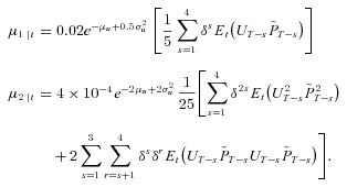
The Moments of the Replacement Rate Distribution

The Earnings Model for Old
 (A1)
(A1)
The Contribution Model for Young
 (A2)
(A2)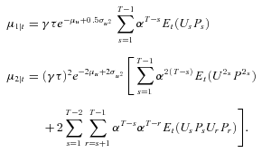
The Model for the Middle-Aged
 (A3)
(A3)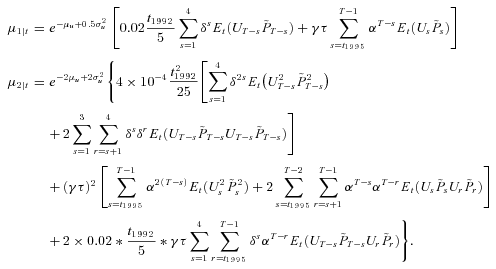
The Survey
The 2006 UCS is a national representative sample of the eligible population of Unicredit customers. The eligible population of customers excludes customers under 20 and over 80, and customers with assets of less than 10,000 euros with Unicredit. The sampled population size is around 1.3 million customers. The survey was aimed at acquiring information on the behavior and expectations of Unicredit Group customers and focused on multibanking, attitude toward saving and investing, financial literacy and propensity for risk, pensions, and insurance requirements.
The sampling scheme is similar to that for the Bank of Italy Survey of Household Income and Wealth (SHIW). The population is stratified along two criteria: geographical area of residence (Northeast, Northwest, Central, and Southern Italy) and wealth held with Unicredit as of June 30, 2006. The sample size is 1,686 customers, of whom 1,580 are from Unicredit Retail Bank and 106 are from Unicredit Private Bank (the upper tier customer bank). The survey was administered between May 1 and September 30, 2007 by a leading Italian polling agency, which also conducts the SHIW for the Bank of Italy. Most interviewers had substantial experience of administering the SHIW, which is likely to increase the quality of the data. The UCS was piloted in the first quarter of 2007, and the Computer Assisted Personal Interview methodology was employed for all interviews. To overcome some of the problems arising from nonresponses, the sample was balanced ex post with respect to the true distribution of assets, area of residence, city size, gender, age, and education of the eligible population.
The questionnaire comprises nine sections. Sections A and B refer, respectively, to respondent and household demographic and occupation variables. Section C focuses on saving, investment, and financial risk. Section D includes detailed questions on financial wealth and portfolio allocation, and Section E inquires about consumer debt and mortgages. By design, Sections A, B, D, and E allow a perfect matching with the SHIW questionnaire. Questions on real estate and entrepreneurial activities are included in Section F. Section G contains questions on subjective expectations, and Section H focuses on insurance and private pension funds. The last two sections ask about income and expectations about and need for insurance and pension products.
Table A1 shows that, compared to Italian households surveyed in the 2006 Bank of Italy SHIW, Unicredit Group customers are slightly older, more educated, less likely to work in the manufacturing sector, and more likely to live in the North. Table A1, column (3) reports statistics for SHIW respondents with a bank account. Although the samples are drawn from different populations, they have similar demographic characteristics. Therefore we do not reweight the sample to make it representative of Italian households with a bank account.
| UCS | SHIW Highest Income Earner | SHIW Bank Account Holder | |
|---|---|---|---|
| Gender | |||
| Male | 0.69 | 0.69 | 0.71 |
| Female | 0.31 | 0.31 | 0.29 |
| Age | |||
| Up to 30 | 0.04 | 0.06 | 0.06 |
| 31 to 40 | 0.18 | 0.19 | 0.20 |
| 41 to 50 | 0.22 | 0.22 | 0.22 |
| 51 to 65 | 0.36 | 0.24 | 0.24 |
| Over 65 | 0.20 | 0.29 | 0.27 |
| Education | |||
| Elementary school | 0.10 | 0.27 | 0.22 |
| Middle school | 0.29 | 0.36 | 0.37 |
| High school | 0.41 | 0.27 | 0.30 |
| University degree | 0.20 | 0.10 | 0.10 |
| Sector of activity | |||
| Agriculture | 0.03 | 0.03 | 0.03 |
| Industry | 0.13 | 0.21 | 0.23 |
| Public sector | 0.19 | 0.15 | 0.17 |
| Other sector | 0.30 | 0.19 | 0.20 |
| Not employed | 0.35 | 0.40 | 0.37 |
| Household size | |||
| 1 member | 0.21 | 0.25 | 0.23 |
| 2 members | 0.29 | 0.28 | 0.29 |
| 3 members | 0.26 | 0.21 | 0.22 |
| 4 members | 0.20 | 0.18 | 0.19 |
| 5 or more members | 0.04 | 0.07 | 0.06 |
| Geographical area | |||
| Northern Italy | 0.73 | 0.48 | 0.52 |
| Central Italy | 0.14 | 0.20 | 0.21 |
| South and Islands | 0.13 | 0.32 | 0.27 |
- a Notes: The table compares sample means of selected demographic variables in the UCS and 2006 SHIW. Means are computed using sample weights.
The Subjective Probability Distribution of the Replacement Rate


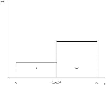
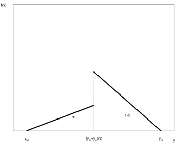
We consider two assumptions concerning f(y). The first is that y is uniformly distributed over each of the two intervals: [ym, (ym + yM)/2] and ((ym + yM)/2, yM]. If π = 0.5, the distribution collapses to a single uniform distribution defined in the interval [ym, yM]. A second possibility is to assume that the distribution is triangular over the same two intervals; if π = 0.5, the distribution collapses to a single triangular distribution over the interval [ym, yM]. Note that in both cases E(y) and Var(y) depend only on the three known parameters (ym, yM, and π). The triangular distribution is a more plausible description of the probability distribution of the replacement rate, because outcomes farther away from the mid-point receive less weight. Figures A1 and A2 show the p.d.f. under the uniform and the triangular assumptions.
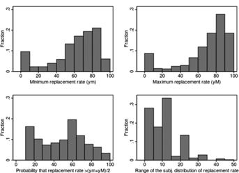
Figure A3 plots the raw data, that is, the subjective distributions of ym, yM, (1 – π), and (yM, ym). Slightly less than 30 percent of respondents report a limited range of the subjective distribution; instead, for 30 percent the range of the replacement rate is between 10 and 15 percent.


