A Combined Monte Carlo and Possibilistic Approach to Uncertainty Propagation in Event Tree Analysis
Abstract
In risk analysis, the treatment of the epistemic uncertainty associated to the probability of occurrence of an event is fundamental. Traditionally, probabilistic distributions have been used to characterize the epistemic uncertainty due to imprecise knowledge of the parameters in risk models. On the other hand, it has been argued that in certain instances such uncertainty may be best accounted for by fuzzy or possibilistic distributions. This seems the case in particular for parameters for which the information available is scarce and of qualitative nature. In practice, it is to be expected that a risk model contains some parameters affected by uncertainties that may be best represented by probability distributions and some other parameters that may be more properly described in terms of fuzzy or possibilistic distributions. In this article, a hybrid method that jointly propagates probabilistic and possibilistic uncertainties is considered and compared with pure probabilistic and pure fuzzy methods for uncertainty propagation. The analyses are carried out on a case study concerning the uncertainties in the probabilities of occurrence of accident sequences in an event tree analysis of a nuclear power plant.
1. INTRODUCTION
An important aspect of quantitative risk analysis lies in the appropriate characterization, representation, propagation, and interpretation of uncertainty, which is an unavoidable element affecting the limit behavior of any engineered system.
Uncertainty is typically considered of two different types: randomness due to inherent variability in the system behavior and imprecision due to lack of knowledge and information on the system. The former type of uncertainty is often referred to as objective, aleatory, stochastic whereas the latter is often referred to as subjective, epistemic state of knowledge (Apostolakis, 1990; Helton, 2004).
The distinction between aleatory and epistemic uncertainty plays a particularly important role in the quantitative risk assessment framework applied to complex engineered systems, such as nuclear power plants, aerospace systems, chemical, and process components. In this context, aleatory uncertainty relates to the occurrence of the events that define the various possible accident scenarios whereas epistemic uncertainty arises from a lack of knowledge of fixed but poorly known parameter values entering the evaluation of the probabilities and consequences of the accident scenarios.
In the current risk assessment practice, both types of uncertainties are represented by means of probability distributions (IAEA, 1992; NASA, 2002; Vose, 2000), and the uncertainty propagation is carried out by a two-loops Monte Carlo simulation where in the outer loop the values of the parameters (e.g., failure rates) affected by epistemic uncertainty are sampled and in the inner loop the aleatory variables (e.g., failure times) are sampled from the probability distributions conditioned at the values of the epistemic parameters sampled in the outer loop (Rao et al., 2007). However, resorting to a probabilistic representation of epistemic uncertainty may not be possible when sufficiently informative data are not available for statistical analysis, even if one adopts expert elicitation procedures to incorporate diffuse information into the corresponding probability distributions, within a subjective view of probability. Indeed, an expert may not have sufficiently refined knowledge or opinion to characterize the relevant epistemic uncertainty in terms of probability distributions (Helton, 2004; Huang et al., 2006).
As a result of the potential limitations associated to a probabilistic representation of epistemic uncertainty under limited information, a number of alternative representation frameworks have been proposed (Ferson & Lev, 1996; Ferson et al., 2004), for example, fuzzy set theory (Zadeh, 1965), evidence theory (Shafer, 1976), possibility theory (Dubois & Prade, 1988), probability bounds, and interval analysis (Moore, 1979).
Fuzzy set theory, in particular, has been recently proposed for risk assessment applications because of its representation power and its relative mathematical simplicity. In the context of fault tree and event tree analyses, basic event probabilities have been treated as trapezoidal fuzzy numbers and the extension principle has been applied to compute the probability of occurrence of the top event or of the accident sequences (Tanaka et al., 1983; Liang & Wang, 1991; Huang et al., 2001). In order to deal with repeated basic events in fault tree analysis, Soman and Misra (1993) provided a simple method for fuzzy fault tree analysis based on the α-cut method, also known as resolution identity. Another interesting approach to fuzzy fault tree analysis based on the treatment of the system state as a fuzzy variable has been proposed by Huang et al. (2004).
In the present article, the problem of the representation and propagation of the epistemic uncertainty associated to the probability of occurrence of events is addressed within the event tree analysis scheme. The approach is based on the joint use of probability and possibility theories for the treatment of the uncertainties regarding the probability of occurrence of the events. Probability theory is well known and extensively applied in event tree analysis; possibility theory is similar to probability theory in that it is based on set functions, but it differs from it in that it makes use of dual set functions called possibility and necessity measures.
With respect to the representation of uncertainty, when sufficiently informative data are available probabilistic distributions are righteously used; in the opposite case, one resorts to the elicitation of expert knowledge that is often of ambiguous, qualitative nature so that the associated uncertainty may be more adequately captured by possibilistic distributions. Examples of events whose uncertain probabilities of occurrence can typically be described by probabilistic distributions are basic hardware failures, whereas for the probabilities of occurrence of human errors or of failures to protective or automation systems possibilistic distributions may be more appropriate.
In general, an event tree may contain events of both kinds. In this article, the propagation of the epistemic uncertainty of these events, represented by both probabilistic and possibilistic distributions, is performed by resorting to a hybrid approach (Baudrit et al., 2006) that combines the Monte Carlo (MC) technique (Kalos & Whitlock, 1986) with the extension principle of fuzzy set theory (Zadeh, 1965). MC sampling of the random variables is repeatedly performed to process the epistemic uncertainty related to the events whose probabilities of occurrence are described by probabilistic distributions and fuzzy interval analysis is carried out at each sampling to process the epistemic uncertainty associated to the events whose probabilities of occurrence are described by possibilistic distributions.
The original contribution of the present study consists in the adaptation of the hybrid approach to event tree analysis and a thorough critical comparison of the results thereby obtained with those obtained by:
- 1
A pure probabilistic approach, based on the transformation of the possibilistic distributions into probabilistic distributions and the successive propagation of the uncertainty via MC sampling (Marseguerra & Zio, 2002).
- 2
A pure fuzzy set approach, based on the transformation into fuzzy numbers of the probabilistic description of the uncertainty on some of the parameters and the successive propagation of all the uncertainties via fuzzy set arithmetic (Huang et al., 2001).
The case study considered for the comparison regards the evaluation of the probabilities of occurrence of the accident sequences developing from an anticipated transient without scram (ATWS) event in a nuclear power plant (Huang et al., 2001).
The article is organized as follows. In Section 2, the hybrid technique for the joint propagation of possibilistic and probabilistic uncertainty through a generic mathematical function is discussed. Section 3 describes the case study considered. In Section 4, the results obtained by applying the hybrid technique are shown and commented while in Section 5 they are compared with the results obtained by the pure probabilistic and pure fuzzy approaches. Conclusions and directions for future work are provided in the last section.
2. JOINT PROPAGATION OF PROBABILISTIC AND POSSIBILISTIC UNCERTAINTY
Let us consider a model whose output is a function f(·) of n input variables Yj, j= 1, … , n; the uncertainty in the first k input variables (hereafter called “probabilistic” variables) is characterized by probability distributions  whereas the uncertainty in the last n−k input variables (hereafter called “possibilistic” variables) is represented in terms of possibility distributions
  measuring the degree of possibility that the linguistic variables Yj be equal to y. For the propagation of such mixed uncertainty information, the Monte Carlo technique (Kalos & Whitlock, 1986) can be combined with the extension principle of fuzzy set theory (Zadeh, 1965) by means of the following two main steps (Baudrit et al. 2006):
- 1
Repeated Monte Carlo sampling of the probabilistic variables to process their uncertainty;
- 2
Fuzzy interval analysis to process the uncertainty connected with the possibilistic variables.
For the generic ithk−tuple of random values, i= 1, 2, … , m, sampled by Monte Carlo from the probabilistic distributions, a fuzzy set πfi estimate of f(Y) is constructed by fuzzy interval analysis. After m repeated samplings of the probabilistic variables, the fuzzy set estimates πfi, i= 1, … , m, are combined to give an estimate of f(Y) as a fuzzy random variable (or random possibility distribution) according to the rules of evidence theory (Shafer, 1976).
The operative steps of the procedure are:
- 1
Sample the ith realization (yi1, … , yik) of the probabilistic variable vector (Y1, … , Yk).
- 2
Select a possibility value α and the corresponding cuts of the possibility distributions
 as intervals of possible values of the possibilistic variables (Yk+1, … , Yn).
 - 3
Compute the smallest and largest values of f(yi1, … , yik, Yk+1, … , Yn), denoted by
 and
and  , respectively, considering the fixed values (yi1, … , yik) sampled for the random variables (Y1, … , Yk) and all values of the possibilistic variables (Yk+1, … , Yn) in the α−cuts of their possibility distributions
  . Then, take the extreme values
  and
and  found in Step 3 as the lower and upper limits of the α− cut of f(yi1, … , yik, Yk+1, … , Yn).
 - 4
Return to Step 2 and repeat for another α-cut; after having repeated Steps 2–3 for all the α-cuts of interest, the fuzzy random realization (fuzzy interval) πfi of f(Y) is obtained as the collection of the values
 and
and  ; in other words, πfi is defined by all its α-cut intervals
  .
. - 5
Return to Step 1 to generate a new realization of the random variables.
 (1)
(1) (2)
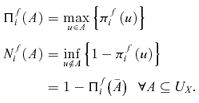
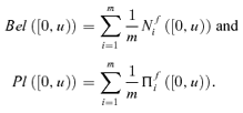
(2)The likelihood of the value f(Y) passing a given threshold u can then be computed by considering the believe and the plausibility of the set A= (−∞, u]; in this respect, Bel(f(Y) ∈ (−∞, u]) and Pl(f(Y) ∈ (−∞, u]) can be interpreted as bounding, average cumulative distributions  (Baudrit et al., 2006).
Let the core and the support of a possibilistic distribution πf(u) be the crisp sets of all points of UX such that πf(u) is equal to 1 and nonzero, respectively. Considering a generic value u of f(Y), it is Pl(f(Y) ∈ (−∞, u]) = 1 if and only if Πfi (f(Y) ∈ (−∞, u]) = 1, ∀i= 1, … , m, that is, for  . Similarly, Pl(f(Y) ∈ (−∞, u]) = 0 if and only if Πfi(f(Y) ∈ (−∞, u]) = 0, ∀i= 1, … , m, that is, for
  .
.
Finally, one way to estimate the total uncertainty on f(Y) is to provide a confidence interval at a given level of confidence, taking the lower and upper bounds from Pl(f(Y) ∈ (−∞, u]) and Bel(f(Y) ∈ (−∞, u]), respectively (Baudrit et al., 2006). On the other hand, Bel(f(Y) ∈ (−∞, u]) and Pl(f(Y) ∈ (−∞, u]) cannot convey any information on the prediction that f(Y) lies within a given interval [u1, u2], since neither Bel(f(Y) ∈[u1, u2]) nor Pl(f(Y) ∈[u1, u2]) can be expressed in terms of Bel(f(Y) ∈ (−∞, u]) and Pl(f(Y) ∈ (−∞, u]), respectively.
3. CASE STUDY
The approach for uncertainty propagation illustrated in Section 2 has been applied to the event tree analysis of an ATWS event in a nuclear power plant in Taiwan (Huang et al., 2001).
3.1. The Event Tree
An ATWS occurs if the protection system diagnoses a potential damage in the plant that requires inserting the control rods into the reactor core to shut down the nuclear reaction, but the operation is unsuccessful. To analyze the sequence of occurrences following the ATWS, the event tree in Fig. 1 is considered, taken from Taiwan's nuclear power plant II operating PRA draft report (PRA Report, 1995). The headings (top events) of the tree are reported in Table I. According to the assumptions made (PRA Report, 1995), the probabilities of occurrence of events XC and V are conditioned by the occurrence of events U1 and X1, whereas the probabilities of events Xv, W, and VW are considered as constants in the different sequences. It is to be noted, however, that the method for uncertainty propagation here proposed could be applied without any restriction also if these assumptions were relaxed.
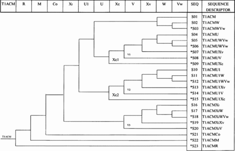
The event tree (Huang et al., 2001); upper branch corresponds to the nonoccurrence of the event, lower branch to the occurrence. SEQ = sequence number; *= severe consequence sequence.
| Event | Acronym | Type | ν | Description |
|---|---|---|---|---|
| Main condenser isolation ATWS | T1ACM | HFD | ν1 | This event will happen when the reactor is isolated and the automatic scram system fails. It is also assumed that mechanical failures cannot be repaired within the allowable time. |
| Recirculation pump trip | R | HFD | ν2 | If the plant fails to scram, an automatic recirculation pump system is required to limit power generation immediately. A failure of the automatic recirculation pump system will result in event R. |
| Safety/relief valves (S/RVs) open | M | HFD | ν3 | At the time the reactor is isolated, at least 13 of 16 S/RVs must open to prevent overpressurization of the reactor vessel. If insufficient S/RVs open, then event M will happen. |
| Boron injection | C 0 | HFD | ν4 | When an ATWS event happens, the power of the core is very high. If the power cannot be slowed down to the state of shutdown, and the vapor produced by the reactor continues to inject into the suppression pool, then the temperature will increase to fail the high-pressure system. This will increase the possibility of core meltdown. As a result, automatic redundant reactivity control system (RRCS) is supposed to inject liquid Boron into the vessel to shut down the reactor safely. If automatic RRCS fails, and operators fail to inject liquid Boron by using standby liquid control system (SLCS), it will result in event C0. It is assumed that operators cannot manually inject liquid Boron within the allowable time. |
| ADS inhibit | X I | HED | ν12 | Automatic depressurization system (ADS) is designed to decrease the pressure of the reactor in order to start the low-pressure system. The low-pressure system will inject water into the reactor vessel to protect the fuel. When an ATWS event happens, the reactor power is controlled by the level of water in core. Since high-level water will cause high power, the operator should inhibit all ADS valves manually. If the operator fails to do so, event XI will occur. |
| Early high-pressure makeup | U1 | HFD | ν5 | Following the stop of feedwater supply, the high-pressure makeup system is supposed to work automatically when automatic actuation alarm appears as soon as the water level is lowering till level 2. The water level is expected to reach the top of the fuel. Thus, if the high-pressure system fails to work automatically, it will lead to event U1. |
| Long-term high-pressure makeup | U | HFD | ν6 | The success criterion of avoidance of this event is that the high-pressure system can maintain the water level in the vessel 24 hours after the start. If the system fails and causes event U, then using the low-pressure system to maintain the water level is needed. |
| Manual reactor depressurization | XC (Xc1,Xc2) | HED | ν13, ν14 | If the pressure in the reactor vessel is too high to set up the low-pressure system, the operator should depressurize the vessel manually in time to avoid core melt-down. Due to the different conditional probabilities of occurrence of this event in different accidental sequences, Xc is called Xc1 in sequences 4–9 characterized by the nonoccurrence of event U1 and XC2 in sequences 10–15 characterized by the occurrence of event U1. |
| Reactor inventory makeup at low pressure | V (V1,V2,V3) | HFD | ν7, ν8, ν9 | If the low-pressure system fails as well as the high-pressure system, then event V will occur and the water level in the vessel will be so low as to probably cause core melt-down. Due to the different conditional probabilities of occurrence of this event in different accidental sequences, V is called V1 in sequences 4–7, V2 in sequences 10–14, and V3 in sequences 16–20. |
| Vessel overfill prevention | XV | HED | ν15 | When the pressure in the vessel is decreased till the level low enough for the low-pressure system to inject water, huge amount of water will come into the core. The operator should pay attention to the water level and make sure that the level is kept not so high as to lead to core melt-down. The definition of this event is the operator fails to complete this job. |
| Long-term heat removal | W | HFD | ν10 | The residual heat removal (RHR) system is initialized to cool down the suppression pool and containment in order to maintain other supporting systems working well. If this system fails, event W will happen. |
| Vessel inventory makeup after containment (CTMT) failure | VW | HFD | ν11 | The CTMT might fail because of overpressure or overheat. The water in the reactor vessel must be kept supplying to protect the fuel not to melt in the condition of CTMT failure. Among these events, XI, XC, and XV are mainly caused by human errors. The others are mainly caused by hardware failures. |
- ν= probability of occurrence; HFD = hardware-failure-dominated; HED = human-error-dominated.
3.2. Estimation of Probability and Possibility Distributions
Two kinds of information are available with respect to the event occurrences in the event tree. Adopting the same assumptions of Huang et al. (2001), sufficient experimental data are available to build lognormal probability distributions  representing the uncertainty in the event probabilities νj, j= 1, … , k, for the k= 11 hardware-failure-dominated (HFD) events (Fig. 2). Table II reports the corresponding means and standard deviations.
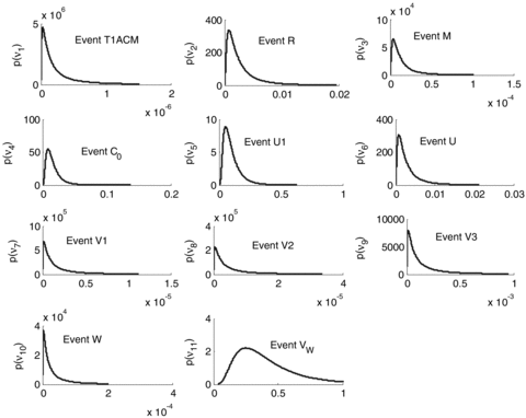
Probability density functions for the probabilities of occurrence of the 11 hardware-failure-dominated events of Table I.
| Event | Median | Error Factor | |
|---|---|---|---|
| T1ACM |  |
1.52E-07 | 8.42 |
| R |  |
1.96E-03 | 5.00 |
| M |  |
1.00E-05 | 5.00 |
| C 0 |  |
1.37E-02 | 3.00 |
| U1 | p ν5(ν) | 8.45E-02 | 3.00 |
| U |  |
2.13E-03 | 5.00 |
| V1 |  |
1.12E-06 | 10.00 |
| V2 |  |
3.40E-06 | 10.00 |
| V3 |  |
9.49E-05 | 10.00 |
| W |  |
2.03E-05 | 10.00 |
| Vw |  |
4.00E-01 | 2.40 |
On the contrary, there are not enough data to build probability distributions for the human-error-dominated events: in this case, the knowledge of four experts has been elicited in the form of possibility distributions  , j= 12, 13, 14, 15 (Fig. 3) (Huang et al., 2001).
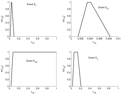
Possibility distributions of the probabilities of occurrence of the four human-error-dominated events of Table I (Huang et al., 2001).
4. UNCERTAINTY PROPAGATION THROUGH THE EVENT TREE BY THE HYBRID MONTE CARLO AND POSSIBILISTIC APPROACH
 , is the product of the probabilities νj of occurrence/nonoccurrence of the single events along the sequence, that is,
 (3)
(3) (4)
(4)
- 1
With respect to the HFD events probabilities ν1, ν2, ν3, ν4, ν5 (the probabilistic variables), m= 1,000 realizations vi1, νi2, νi3, νi4, νi5, i= 1, … , 1,000 have been sampled from the corresponding probability density functions of Fig. 2. Then, for each realization, Steps 2–4 below have been performed.
- 2
With respect to the human-error-dominated (HED) events probabilities ν12, ν14 (the possibilistic variables), 20 values of α (0.05, 0.1, … , 1) have been considered. The α-cuts
 and
and  of the corresponding possibilistic distributions π(ν12) and π(ν14) have been found and for each α-cut, Steps 3–5 below have been performed. For the ith realization of the probabilistic variables and the α-cut of the possibilistic variables, the smallest
  and largest
  values of f15 have been computed considering the fixed values vi1, νi2, νi3, νi4, νi5 and all values of ν12 and ν14 in their α-cut intervals
  and
and  . In this particular case, given the structure of f15,
  and
and  . The lower and upper limits of the α-cut of f15 for the ith realization are, respectively,
  and
and  .
. - 3
After having repeated Step 3 for all the 20 α-cuts found in Step 2, the fuzzy random realization πfi of f(Y) is constructed as the collection of its 20 α-cut intervals
 .
. - 4
Steps 2–4 have been repeated for each of the m= 1,000 realizations vi1, νi2, νi3, νi4, νi5, i= 1, … , 1,000, giving m fuzzy random realizations πfi. Fig. 4 (top) shows two different examples of fuzzy random realizations of the probability of occurrence of accident sequence 15.
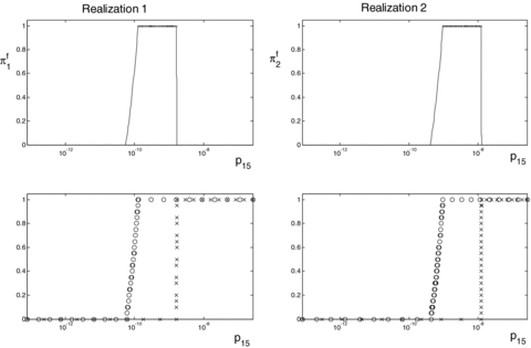
Top: two different fuzzy random realizations of the probability of occurrence of accident sequence 15. Bottom: corresponding necessity (o) and possibility (x) measures.
Then, for all sets A=[0, u), u∈R+, the possibility and the necessity measures, Πfi ([0, u)) and Nfi ([0, u)), are obtained from the corresponding possibility distributions πfi(u), according to Equation (1). Fig. 4-bottom reports the possibility and necessity measures corresponding to the possibility distributions shown in Fig. 4-top.
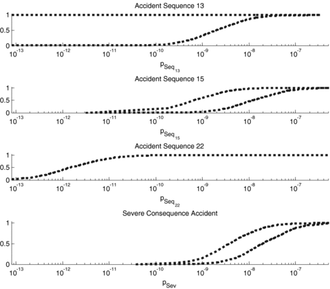
Believe and plausibility of the set [0,u) resulting from application of the hybrid approach.
In the top graph, notice that the Bel([0, u)) (lower curve) and the Pl[0, u) (upper curve) of the probability of sequence 13 are quite far from one another, indicating large imprecision in the estimation of the probability that p13 < u, that is, of the cumulative distribution function F(u). This is mainly due to the fact that sequence 13 is characterized by the nonoccurrence of the HED event Xc2 that is known only with very large imprecision (bottom left graph in Fig. 3). For example, the value of Pl(0), which represents the plausibility of the impossibility of the occurrence of accident sequence 13, is equal to 1 while the Bel(0) that represents the necessity is equal to 0. The plausibility measure is 1 due to the fact that the possibility of having ν14= 1 is 1, that is, the expert believes that it is possible that event Xc2 always occurs; on the contrary, event Xc2 appears in sequence 13 as not occurring, so that it is plausible that sequence 13 never occurs  .
.
The opposite occurs for the case of sequence 22, characterized by the occurrence of only HFD events. In this case, the input (probabilistic) variables ν1, ν2, of function f22 are represented by probabilistic distributions not affected by imprecision and thus Bel([0, u)) and Pl([0, u)) coincide and can be interpreted as the cumulative distribution function F(u) (third graph from the top in Fig 5).
An intermediate situation between the cases of sequences 13 and 22 is represented by sequence 15 (second graph from the top of Fig. 5). In this case the estimation of the probability of occurrence of the accident sequence, characterized by the presence of both HED and HFD events, is affected by both imprecision and variability represented by the gap between Bel([0, u)) and Pl([0, u)), and the slopes of the two curves, respectively.
5. COMPARISON WITH OTHER METHODS FOR UNCERTAINTY PROPAGATION
The results of the uncertainty propagation by the hybrid approach have been compared with those obtained by a pure probabilistic and a pure fuzzy propagation.
5.1. Probabilistic Propagation
 (5)
(5)Simple Monte Carlo simulation has then to be used to compute the probabilities of occurrence of the accident sequences. In each Monte Carlo trial, the probabilities of event occurrence are sampled from the corresponding probability density functions and the probability of the accident sequences are then obtained by simple algebraic multiplication of the sampled probabilities of event occurrences along the sequences. From the repetition of m MC sampling trials, empirical distribution functions for the probabilities of the accident sequences are obtained. As an example, Fig. 6 shows the empirical cumulative distribution functions obtained with m= 106 samplings for the accident sequences 13, 15, 22, and for the severe consequence accident probability.
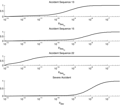
Cumulative distribution functions of the probabilities of accident sequences 13, 15, 22, and of a severe consequence accident resulting from the probabilistic approach.
5.2. Fuzzy Propagation
Dually to the probabilistic approach, the fuzzy approach entails that all parameter uncertainties be described in terms of fuzzy sets, including the HFD events parameters.
The fuzzy approach applied in this article is taken from Huang et al. (2001). First of all, the probability density functions that describe the HFD events have been transformed into triangular fuzzy numbers, peaked (membership equal to 1) at the mean value of the corresponding probability density functions and with the two vertexes of the base (membership equal to 0) positioned in correspondence of the 5% and 95% percentiles. Other techniques for the transformation of probability density functions into fuzzy numbers exist but their investigation is outside the scope of the present study: the interested reader should refer to Klir and Yuan (1995) and Dubois et al. (2004) for some proposed techniques, for example, the bijective transformation.
The probabilities of occurrence of the accident sequences are then computed by fuzzy number multiplication performed using the α-cut method. In particular, only the 20 α-cuts (0.05, 0.1, … , 1) reported in Huang et al. (2001) have been considered, together with the 0 α-cuts (the supports of the fuzzy numbers), which are not given in that study and have been obtained in this study by simple interpolation of the available α-cut values. It is also interesting to note that the approximation introduced by performing the multiplication of triangular or trapezoidal fuzzy numbers by using the α-cut method is not critical for the purpose of this study of comparing different methods for uncertainty propagation.
The obtained membership functions of the probabilities of occurrence of sequences 13, 15, 22, and of a severe consequence accident are reported in Fig. 7.
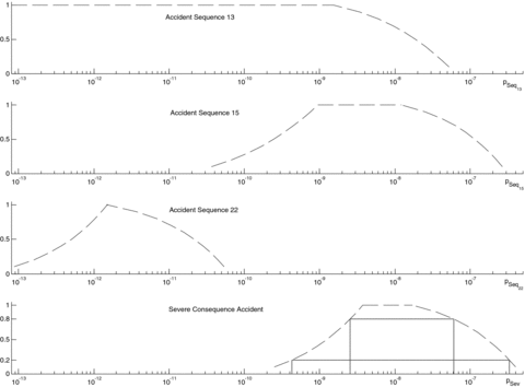
Fuzzy numbers of the probability of sequences 13, 15, 22, and (bottom) of all the sequences that lead to a severe consequence accident. In the bottom graph, α-cuts 0.8 and 0.2 are also depicted.
To eventually compare these results with the previous ones, the fuzzy numbers of Fig. 7 can be interpreted as possibility distributions, that is, the membership functions that define the fuzzy numbers represent the degree of possibility  that
that  is equal to p. In this case, the possibility measures
  and the necessity measures
  associated to the possibilistic distributions are given by Equation (2). Then, the believe and the plausibility functions, Bel([0, u)) and Pl([0, u)), represented in Fig. 8 can be obtained, following the procedure of Section 2.
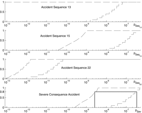
Believe Bel(n[0, u)) and plausibility Pl([0, u)) lower and upper curves, respectively, obtained from the fuzzy numbers of Fig. 7. The interval of possible values for the 0.8 upper confidence bound is also depicted.
Notice that Figs. 7 and 8 present the same information under two different points of view: the fuzzy numbers of the former figure can be read in terms of α-cuts, while the believe and plausibility functions of the latter figure can be interpreted by fixing a level of confidence and providing an interval of possible values for the one-sided upper limit by taking the upper and lower bounds from Bel([0, u)) and Pl([0, u)). For example, the α-cut 0.8 of the severe accident probabilities is (2.549·10−9, 6.056·10−8) and the α-cut 0.2 is (4.261·10−10, 3.322·10−7), whereas the 80% one-sided upper limit of the severe consequence accident probabilities lies between (2.549·10−9, 6.056·10−8). Thus, the a/100 one-sided upper limit can have values between the left limit of the α-cut a and the right limit of the α-cut (1 –a). This is due to the definition of plausibility and belief measures given by Equation (1) from which we get that the value u1 such that Pl(0, u1) =a corresponds to the left limit of the α-cut a, that is, the minimum value of X with a possibility of a, while the value u2 such that Bel(0, u2) =a corresponds to the right limit of the α-cut (1 –a). In particular, the believe function reaches 1 in correspondence of the right limit of the support.
5.3. Comparison of the Methods
8-11 show the comparison of the cumulative distributions obtained by the probabilistic uncertainty propagation approach with the believe and plausibility functions obtained by the fuzzy and hybrid approaches.
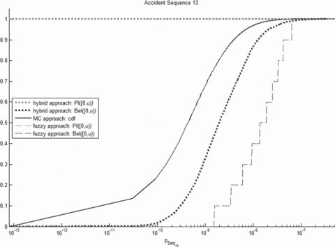
Comparison of the cumulative distribution functions of the probability of occurrence of accident sequence 13 obtained by the probabilistic uncertainty propagation approach with the believe and plausibility functions, Bel([0, u)) and Pl([0, u)), obtained by the fuzzy and hybrid approaches (possibility functions obtained by the hybrid and fuzzy approaches are in this case completely overlapping).
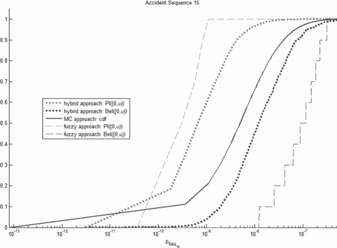
Comparison of the cumulative distribution functions of the probability of occurrence of accident sequence 15 obtained by the probabilistic uncertainty propagation approach with the believe (lower curve) and plausibility (upper curve) functions, Bel([0, u)) and Pl([0, u)), obtained by the fuzzy and hybrid approaches.

Comparison of the cumulative distribution functions of the probability of occurrence of accident sequence 22 obtained by the probabilistic uncertainty propagation approach with the believe (lower curve) and plausibility (upper curve) functions, Bel([0, u)) and Pl([0, u)), obtained by the fuzzy and hybrid approaches.
5.3.1. Comparison Between the Hybrid and the Probabilistic Approach
In the case of the computation of the probability of sequence 22, characterized by input parameters whose uncertainty is represented only by probabilistic distributions, the hybrid and the probabilistic approaches coincide. The small differences between the cumulative distribution function obtained by the probabilistic approach and the believe and plausibility functions in Fig. 11 is due to the different number of samplings, m, that have been performed for the probabilistic estimation (m= 106) and for the hybrid approach estimation (m= 1,000).
The computation of the probability of sequence 13 is characterized by the presence of the HED event Xc2. The knowledge of the probability of occurrence of this event is affected by a large amount of imprecision given that the analyst gives a degree of possibility of 1 to all probabilities of occurrence from 0.1 to 1. With the hybrid approach, the uncertainty on this possibilistic input variable is reflected in a large amount of imprecision of the probability of sequence 13. For example, the probability that pSeq13 < 1 · 10−13 can go from 0 to 1 (believe and plausibility functions of the set [0, 1 · 10−13)). Completely different is the case of the probabilistic approach where the possibility distribution of the Xc2 probability of occurrence is firstly transformed into a probability density function. This transformation causes, for example, that the probability of having a value of probability of occurrence of Xc2 larger than 0.99 is equal to 0.011 (while the possibility of the same event is 1). This results in a very low value (0.005) of the probability of having pSeq13 < 1 · 10−13.
The case of sequence 15 (Fig. 10) is intermediate between the cases of sequences 13 and 22, since the propagation of the uncertainty in the occurrence of the HED event Xc2 still causes a separation between the believe and the plausibility functions, but in reduced terms if compared to the case of sequence 13.
To sum up the comparison, if at least one input parameter is described by a possibilistic distribution (cases of sequences 13 and 15), the hybrid approach more explicitly propagates the uncertainty by separating the contributions coming from the probabilistic and possibilistic variables; this separation is visible in the output distributions of the accident sequence probabilities where the separation between Bel([0, u)) and Pl([0, u)) reflects the imprecision in the knowledge of the HFD events, whereas the uncertainty in the output distribution of the pure probabilistic approach is given only by the slope of the cumulative distribution. Furthermore, note that the cumulative distribution of the accident sequence probability obtained by the pure probabilistic method is within the believe and plausibility functions obtained by the hybrid approach.
5.3.2. Comparison Between the Hybrid and the Fuzzy Approach
The believe and plausibility functions obtained by the fuzzy approach are in all cases further away from each other than in the case of the hybrid Monte Carlo and possibilistic approach (8-11). This is due to the fact that within the fuzzy approach all the input probabilities are described by possibilistic distributions while in the possibilistic approach only the HED event probabilities of occurrence are described this way. In particular, notice that the difference between the believe and plausibility curves obtained by the two approaches is more remarkable in the case of sequence 22 characterized only by HFD events than in the case of sequence 13, in which the uncertainties due to the HED events are predominant. The probability of occurrence of sequence 15 (Fig. 10) is characterized by the fact that for values of u lower than 2 · 10−10 the plausibility Pl([0, u)) obtained by the fuzzy approach is lower than the plausibility obtained by the hybrid approach. This effect depends from the transformation done in the fuzzy approach of the lognormal probability density functions into triangular fuzzy numbers that completely neglect the possibility to have probability values lower than the 5th percentile or higher than the 95th percentile of the original lognormal probability distributions. This approximation serves only the purpose of the comparison but may be considered critical because it is not conservative in the sense of risk analysis.
It is also interesting to observe that in a hypothetical limit case of function f affected only by possibilistic epistemic uncertainty, the two approaches would lead to the same result.
For what concerns the variability of the output probability due to the epistemic uncertainties in the HFD events that is represented by the slope of the believe and plausibility curves, 8-11 show that, as expected, the hybrid approach generates less-steep believe and plausibility curves than the pure fuzzy approach. This effect is particularly visible in the parts of the curves of Fig. 12 with low believe and plausibility values.
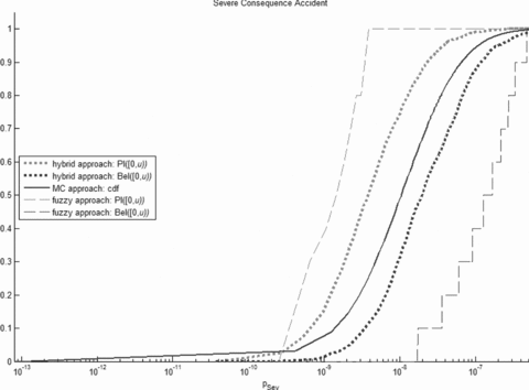
Comparison of the cumulative distribution functions of the probability of occurrence of a severe consequence accident obtained by the probabilistic uncertainty propagation approach with the believe (lower curve) and plausibility (upper curve) functions, Bel([0, u)) and Pl([0, u)), obtained by the fuzzy and hybrid approaches.
5.3.3. Comparison of the Results for the Probability of Occurrence of a Severe Consequence Accident
To interpret the results for the probability of occurrence of a severe consequence accident, confidence intervals are taken from the believe and plausibility functions Bel([0, u)) and Pl([0, u)). For example, in Table III it is shown that the one-sided 95% upper limit obtained by the hybrid approach can be between (3.78·10−8, 1.95·10−7). Notice that the upper bound (1.95·10−7) is only slightly larger than the one-sided upper limit obtained by the probabilistic approach (1.09·10−7), whereas the interval obtained by the fuzzy approach is much larger (3.84·10−9, 4.00·10−7).
| One-sided upper limit | 95% |
| Hybrid approach | (3.78·10−8, 1.95·10−7) |
| Probabilistic approach | 1.09·10−7 |
| Fuzzy approach | (3.84·10−9, 4.00·10−7) |
With respect to the hybrid approach, it is remarkable that the size of the interval within which the upper limit can lie results only from the epistemic uncertainty affecting the knowledge of the HED events. Thus, if the risk analyst were interested in reducing the imprecision on the estimation of the one-sided upper limit, he or she should try to reduce the imprecision regarding the characterization of the probability of occurrence of the HED events.
6. CONCLUSIONS
In this article, the important issue of propagating uncertainty in quantitative risk analysis has been addressed by a hybrid Monte Carlo and possibilistic approach and the results obtained in an application to event tree analysis have been compared with those of a pure probabilistic approach and a pure fuzzy approach.
The case study considered in the application regards the evaluation of the probabilities of occurrence of the accident sequences of an event tree of an ATWS event. Two different types of representation of the epistemic uncertainty have been considered to characterize the knowledge on the event occurrences in the event tree: probabilistic variables with respect to the probability of occurrence of the HFD events for which experimental test data are available and possibilistic variables with respect to the probability of occurrence of the HED events for which expert knowledge can be elicited.
The application of the pure probabilistic approach, based on the description of the event probability of occurrence in terms of probability density functions, has resulted in probability distributions that do not fully catch the imprecision typically affecting the HED events. Conversely, the application of the pure fuzzy approach, based on the description of the probability of occurrence of the events in terms of fuzzy numbers, seems not satisfactory in the propagation of the epistemic uncertainty affecting the HFD events resulting in too imprecise fuzzy sets.
On the contrary, the hybrid approach, based on the combination of the Monte Carlo method with fuzzy interval analysis, has been shown capable of jointly propagating in a satisfactory explicit way the uncertainties characterized by both probabilistic and possibilistic distributions. In particular, the application of the method results in the estimation of upper and lower cumulative distributions of the probabilities of occurrence of the accident sequences, while effectively distinguishing between the uncertainties due to events whose probability of occurrence is described by probabilistic or possibilistic distributions: the former are reflected by the slope of the believe and plausibility functions while the latter are pictured in the gap between the two functions.
A word of caution is in order with respect to the independence assumptions underlying the Monte Carlo sampling and fuzzy interval analysis procedures. First of all, the propagation method proposed assumes stochastic independence between the group of probabilistic variables (Y1, … , Yk) and the group of possibilistic variables (Yk+1, … , Yn), the latter viewed as forming a random Cartesian product on the space of possibilistic variables. Also, a strong dependence between the information sources supplying the different possibility distributions  is assumed, since the same confidence level is used to build the α-cuts. These issues are worth further investigation both from the theoretical and practical points of view.
ACKNOWLEDGMENTS
This study has been carried out with the support of the project Virthualis (FIS5-1999-00250) funded by the European Union.
ACRONYMS AND SYMBOLS
| ATWS | Anticipated transient without scram |
| BWR | Boiling water reactor |
| MC | Monte Carlo |
| ET | Event tree |
| HFD | Hardware-failure-dominated |
| HED | Human-error-dominated |
| Cdf | Cumulative distribution function |
| Probability density function | |
| f(·) | Function through which uncertainty is propagated |
| n | Total number of input variables |
| Yj | jth input variable, j= 1, … , n |
| k | Number of random input variables (k≤n) |
 |
Probability density function of random input variable Yj, j= 1, … , k |
| (yi1, … , yik) | ith realization of the random variable vector (Y1, … , Yk) |
| pi | Probability of sampling the ith realization (yi1, … , yik) of the random variable vector (Y1, … , Yk) |
| m | Number of MC trials |
 |
Possibilistic distribution of input variable Yj, j=k+ 1, … , n |
| X | Output variable |
| UX | Universe of discourse of the output variable X |
| P(X) | Power set of X |
| A | Set of X |
| Π (A) | Possibility measure of A |
| N(A) | Necessity measure of A |
| Bel(A) | Belief measure of A |
| Pl(A) | Plausibility measure of A |
| πf (u) | Possibilistic distribution of the output variable X |
| Core (πf(u)) | Crisp sets of all points of X such that πf(u) is equal to 1 |
| Support (πf(u)) | Crisp sets of all points of X such that πf(u) is nonzero |
 |
Lower mean cumulative distribution of the output variable |
 |
Upper mean cumulative distribution of the output variable |
| νj | Probability of occurrence of the jth event |
 |
Probability of occurrence of the rth accident sequence |
| pSev | Probability of occurrence of a severe consequence accident |


