
Properties of Model-Averaged BMDLs: A Study of Model Averaging in Dichotomous Response Risk Estimation
Abstract
Model averaging (MA) has been proposed as a method of accounting for model uncertainty in benchmark dose (BMD) estimation. The technique has been used to average BMD dose estimates derived from dichotomous dose-response experiments, microbial dose-response experiments, as well as observational epidemiological studies. While MA is a promising tool for the risk assessor, a previous study suggested that the simple strategy of averaging individual models' BMD lower limits did not yield interval estimators that met nominal coverage levels in certain situations, and this performance was very sensitive to the underlying model space chosen. We present a different, more computationally intensive, approach in which the BMD is estimated using the average dose-response model and the corresponding benchmark dose lower bound (BMDL) is computed by bootstrapping. This method is illustrated with TiO2 dose-response rat lung cancer data, and then systematically studied through an extensive Monte Carlo simulation. The results of this study suggest that the MA-BMD, estimated using this technique, performs better, in terms of bias and coverage, than the previous MA methodology. Further, the MA-BMDL achieves nominal coverage in most cases, and is superior to picking the “best fitting model” when estimating the benchmark dose. Although these results show utility of MA for benchmark dose risk estimation, they continue to highlight the importance of choosing an adequate model space as well as proper model fit diagnostics.
1. INTRODUCTION
Risk assessors are often interested in estimating a population's excess risk based upon exposure to a hazardous agent. Alternatively, the exposure level or dose that is related to some prespecified risk level may be of interest. This estimate is frequently based upon the results of fitting a model to the observed data. Commonly, a number of competing models can fit a particular set of data resulting in a range of risk estimates. These estimates are frequently ignored once a single model has been chosen. Although many risk assessors may report a range of risk estimates as an acknowledgment of model uncertainty, the uncertainty in the model selection process is not fully incorporated in most risk assessments.
Some work has been done in incorporating this model uncertainty in risk estimation. Model averaging (MA) has been used in a wide variety of risk assessment contexts. Kang et al.(1) looked at MA in microbial risk assessment; Moon et al.(2) extended this work using a different averaging criterion. Bailer et al.(3,4) used MA in toxicologically based experiments, and Morales et al.(5) looked at Bayesian MA in observational epidemiological studies. In these cases, MA was used as a tool that combined model-specific benchmark dose (BMD) estimates into one central estimate. This risk estimate was formed through a weighted average of each individual model's BMD. Wheeler and Bailer(6) studied MA in the context of toxicologically based risk assessment through a simulation experiment and found that model averaging was typically better for estimating the true BMD than estimates derived from existing model selecting heuristics. Despite this, some questions remained about the appropriateness of the construction of the lower confidence bound on the BMD as well as the construction of the model-averaged BMD estimate itself.
Consequently, we investigate estimating BMDs using an alternative MA technique based on the averaged model. This procedure estimates risk based upon the averaged model and not the average of each model's risk estimates, as was done by Kang et al.,(1) Moon et al.,(2) and Bailer et al.(3,4) This is studied using a simulation experiment designed to mimic risk estimation based upon animal toxicity studies where some dichotomous outcome (death, tumor response, etc.) is recorded.
2. METHODS
2.1. Risk Estimation and the Benchmark Dose
 ((2.1.1))
 ((2.1.2))
 ((2.1.3))
 ((2.1.4))
 ((2.1.5))
 ((2.1.6))
 ((2.1.7))
 ((2.1.8))
 ((2.1.9))
 ((2.1.10))
2.2. Model Averaging
Models (2.1.1)–(2.1.9) frequently produce different BMD estimates from which there is often no reason to prefer one estimate over the other; consequently, uncertainty in BMD estimation results. For example, all models might yield a Pearson χ2 goodness-of-fit statistic with large p-values, and thus there may be little justification in terms of selecting the model solely on model fit. Model averaging takes into account model uncertainty by incorporating results from all models into the estimation process through a weighted average of the model-specific BMD estimates. This technique has been applied in a general modeling context by Raftery,(9) who suggested the use of the posterior model probabilities as weights derived from a Bayesian analysis of all models considered. As a full Bayesian analysis is frequently computationally burdensome, Buckland, Burnham, and Augustin(10) proposed simpler methods, where weights are based upon the penalized likelihood functions formed from the AIC(11) and BIC.(12) The AIC and the BIC are defined as penalized likelihood functions where the AIC =−2 logL+ 2p and the BIC =−2 log(L) +p log(n), and p is the number of parameters in the model, L is the maximum likelihood value, and n represents the sample size. We describe model averaging in the same manner as Buckland et al.,(10) and our work differs from Morales et al.(5) as they use a Bayesian analysis where priors on both the models considered and on the parameters of each of these models were fully specified in the MA.
 formed as a weighted average of K model-specific dose-response estimate
  for k = 1, … , K. Formally this is represented as
  , where
  represents the probability of adverse response given the dose d using the kth model,
  is the estimated parameter vector for the kth model (e.g.,
  for Model (2.1.5)) and wk represents the corresponding weight for the kth model. Given the model Mk in the model space that includes K models, the weight wk is calculated according to the following formula:

Given the estimated function  and a BMR (e.g., values of 1%, 5%, and 10%), the excess risk Model (2.1.10) can be solved to find the corresponding model averaged BMD. As a result of this construction, we describe this as an “average-model” MA estimate for the BMD. As a closed form equation may be unavailable, numerical root-finding methods are used to approximate the BMD. For this work the method of bracketing and bisection(13) is used to compute the benchmark dose. Further, the 100(1 −α)% lower bound benchmark dose estimate is then found using a parametric bootstrap.(14,15) For this study, 2,000 parametric bootstrap resamples are obtained on the central estimate
  ; and for each resample the models are refit to the data, the weights recalculated given this fit, and the “average-model” BMD is computed from this new model average. From these 2,000 “averaged model” BMD estimates a quantile of the bootstrap distribution is found that corresponds to the percentile point α, and this value is used as an estimate for the lower bound on the benchmark dose (BMDL). Here, a 95% BMDL would correspond to the selection of the 5th percentile from the distribution of BMDs from the bootstrap resamples.
The “average-model” MA procedure, and corresponding benchmark dose calculation, does differ significantly from the estimates produced by Kang et al.(1) and Bailer et al.(3,4) They averaged the individual model's BMD and corresponding lower confidence estimates. Thus, given the kth model's benchmark dose estimate and 100(1 −α)% lower bound estimate, the BMDk and BMDLk respectively, the MA BMD estimate is computed as 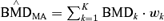 , with the lower bound being computed by as
  . This could be thought of as an “average-dose” MA for BMD estimation. We illustrate the difference in these two methods in application to titanium dioxide rat lung tumor data.
3. APPLICATION TO TITANIUM DIOXIDE RAT LUNG TUMOR DATA
Titanium dioxide (TiO2) is an insoluble powder used in a wide variety of industrial applications, including food, plastics, and paint. Although TiO2 is frequently used as a negative control in animal toxicity studies, the National Institute for Occupational Safety and Health classified TiO2 as a potential occupational carcinogen based upon the observation of lung tumors in rats exposed to high doses.(16,17) As the manufacture of TiO2 may result in high levels of occupational exposure to respirable dust, the risk associated with such exposures is an important occupational health question. If we assume no mechanistic reason to select a particular model form in advance, K= 9 models [i.e., (2.1.1)–(2.1.9) with the multistage Model (2.1.4) having up to a cubic term in the model] were fit to the available data from the experiments of Lee,(16) Muhle et al.,(18) and Heinrich et al.(19) We illustrate the BMD estimation based upon the “average-dose” and “average-model” MA methods using the TiO2 data (Table I).
| Area Dose (m2/g) TiO2 Particle Surface | Tumor Proportion |
|---|---|
| 0 | 3/100 |
| 0 | 1/217 |
| 0 | 2/79 |
| 0 | 0/77 |
| 0.02 | 2/100 |
| 0.03 | 2/71 |
| 0.07 | 1/75 |
| 0.18 | 1/75 |
| 0.28 | 0/74 |
| 1.16 | 13/74 |
| 1.20 | 12/77 |
| 1.31 | 19/100 |
Table II describes the BMDs associated with extra risks of 1% and 10% for Models (2.1.1)–(2.1.9), the model averaged benchmark dose, the AIC, as well as the weights associated with the AIC. For the 10% BMR the quantal-linear dose-response model estimated the BMD as 0.8 m2/g with a 95% lower bound being estimated at 0.6 m2/g; several other models estimate the BMD to be near 1.04 m2/g with the BMDL being estimated in the range of 0.83 to 0.85 m2/g. For 1% excess risk, the quantal-linear model again produces the lowest BMD of 0.08 m2/g and BMDL of 0.06 m2/g. Other models, which arguably describe the data better, as measured by the AIC and goodness-of-fit statistics, estimate the BMD to be around four to five times greater than the quantal-linear model with estimated BMD values around 0.5 m2/g, and corresponding BMDLs estimates between 0.14 and 0.28 m2/g. As there is a significant discrepancy between the estimates at 1%, a central estimate accounting for uncertainty may be desirable.
| Weights | AIC | χ2 GOF p-value | Extra Risk BMD (BMDL) | ||
|---|---|---|---|---|---|
| 10% | 1% | ||||
| Quantal-quadratic | 0.192 | 364.95 | 0.57 | 0.96 | 0.30 |
| (0.84) | (0.26) | ||||
| Logistic | 0.154 | 365.39 | 0.50 | 1.01 | 0.25 |
| (0.92) | (0.21) | ||||
| Probit | 0.134 | 365.66 | 0.48 | 0.97 | 0.22 |
| (0.87) | (0.18) | ||||
| Log-probit | 0.129 | 365.74 | 0.55 | 1.01 | 0.51 |
| (0.79) | (0.20) | ||||
| Gamma | 0.119 | 365.90 | 0.53 | 1.03 | 0.52 |
| (0.83) | (0.18) | ||||
| Log-logistic | 0.112 | 366.03 | 0.52 | 1.04 | 0.50 |
| (0.82) | (0.18) | ||||
| Weibull | 0.108 | 366.11 | 0.52 | 1.04 | 0.49 |
| (0.83) | (0.17) | ||||
| Multistage | 0.039 | 368.11 | 0.61 | 1.04 | 0.47 |
| (0.85) | (0.14) | ||||
| Quantal-linear | 0.013 | 370.35 | 0.26 | 0.80 | 0.08 |
| (0.62) | (0.06) | ||||
| “Average-model” model | n/a | n/a | n/a | 1.01 | 0.36 |
| averaging BMD (BMDL) | (0.82) | (0.12) | |||
| “Average-dose” model | n/a | n/a | n/a | 1.00 | 0.38 |
| averaging BMD (BMDL) | (0.84) | (0.20) | |||
Model averaging can be used to find a central estimate in relation to the model uncertainty described above. The “average-model” MA estimates of the BMD results in benchmark dose estimates of 1.01 m2/g and 0.36 m2/g with 95% BMDLs of 0.82 m2/g and 0.12 m2/g for excess risk of 10% and 1%, respectively. In contrast, the “average-dose” MA estimates of the BMD, i.e., averaging the model-specific BMD estimates as described by Bailer et al.,(3,4) produces BMD estimates of 1.00 m2/g and 0.38 m2/g with 95% BMDLs of 0.84 m2/g and 0.20 m2/g for the BMRs of 10% and 1%, respectively. For the TiO2 cancer dose-response data, these two model averaging methods produce similar BMD point estimates; however, at the 1% level the methods diverge as their BMDL estimates differ by a factor of two. The result is consistent with previous simulation results, which suggest that the BMDL estimated by the “average-dose” method was often very close to the estimated BMD and failed to cover the true BMD at a rate greater than the specified value, and this discrepancy was greater for BMRs of 1%.(6) Even though the “average-model” MA estimate of the BMD provides smaller BMDLs, the behavior/statistical properties of the interval estimator are unknown. Consequently, we study this model averaging technique through a Monte Carlo simulation study.
4. SIMULATION STUDY
In an effort to better understand the proposed “average-model” MA procedure for estimating BMDs, a Monte Carlo simulation study was conducted. To allow for a comparison with the “average-dose” MA method of Kang et al.(1) and Bailer et al.,(3,4) the simulation was carried out using the same conditions as Wheeler and Bailer.(6) While we briefly summarize these conditions below, we refer the reader to Wheeler and Bailer(6) for a more extensive description of the simulation conditions. For the current study, as with previous work, we consider two experimental designs assuming 4 and 6 dose groups, which are spaced geometrically at the design points (0.0, 0.25, 0.5, 1.0) and (0.0, 0.0625, 0.125, 0.25, 0.5, 1.0). For both designs 50 “animals”/experimental units were assigned to each dose group resulting in a sample size of n= 200 for the four-dose-group design and n= 300 for the six-dose-group design. Given a true dose-response curve πTRUE(d), a function representing the probability of response given the dose d, the experiment was simulated and the dichotomous adverse response (e.g., death, tumor response) was generated and recorded.
The true dose-response curve, πTRUE(d), was obtained using the fits of dose-response curves from Models (2.1.1)–(2.1.9) to dose-response data that had a high, medium, and low dose response as well as low and high background response rates. As in Wheeler and Bailer,(6) we considered six dose-response patterns covering two background response conditions crossed with three dose-response steepness conditions (see Table III). These underlying response patterns allowed for curvature that ranged from sublinear to linear dose-response patterns. Given the six response patterns and nine dose-response models, a total of 54 different conditions were used in the simulation. Assuming the true dose-response curve, described above, the simulation proceeded under the assumption that the responses were binomially distributed with n= 50 trials each having the probability of response πTRUE(d), where d represents the dose design points listed above. Thus, the simulation consisted of a set of dose-response curves being fit to the data with the corresponding MA-BMD as well as the MA-BMDL being estimated and recorded. We note that there were random experiments generated through the simulation and bootstrap resampling where it is not possible to estimate a BMD, i.e., the BMD estimate is infinite due to a flat dose-response curve. While such a data set may not be appropriate for risk estimation, it cannot be dismissed in a bootstrap. These values are assigned an arbitrarily large value and reported in the simulation. Consequently, we look at the estimates using the median as a measure of central tendency.
| Response Pattern | Response Curvature |
|---|---|
| 1 | (2%, 7%, 20%) |
| 2 | (2%, 14%, 34%) |
| 3 | (2%, 25%, 50%) |
| 4 | (7%, 12%, 25%) |
| 5 | (7%, 21%, 41%) |
| 6 | (7%, 32%, 55%) |
As previous results have suggested that the variety of the models considered for model averaging is important, two model spaces were considered. The two different model spaces consist of flexible models including the multistage (2.1.4), the Weibull (2.1.9), and the log-probit (2.1.6), and another model space that added the quantal-linear (2.1.7), the quantal-quadratic (2.1.8), the logistic (2.1.1), and the probit (2.1.5) model to the three-model space. This allowed us to study the effects of the models included in the MA on the estimation of the benchmark dose. We note that the log-logistic (2.1.2) and the gamma (2.1.3) models were not used in either model space as the fitting of these models increased the amount of CPU time required, which would make the full simulation intractable. This, however, does not detract from the study as the exclusion of these models allows one to study the utility of model averaging when the true dose-response is not used in the computation.
Given the selected model space (3 or 7 models that are to be averaged) and the true underlying model, 2,000 simulated experiments were generated and the “average-model” MA procedure was applied yielding the MA BMD. Two thousand bootstrap resamples for each of the 2,000 simulated experiments were constructed for estimating the BMDL, and a simple percentile-based estimate of the BMDL was constructed. A separate simulation was conducted for each BMR considered because we are interested in estimating the dose associated with some specified excess risk for BMRs of 1% and 10%.
The simulation, which included the maximum likelihood estimation routines, was written in C++.(20) The GNU Scientific Library,(21) version 1.7, was utilized for all numerical routines; excluding the optimization routines, here the FORTRAN routine dmngb(22) was used for the actual optimization. This software was further checked against the US EPA benchmark dose software by comparing the fits of Models (2.1.1)–(2.1.9) on 2,000 randomly created data sets. Here, the maximum value of the log-likelihood was found to agree in most of the cases. Where the results failed to agree differences within the maximum log-likelihood were small, typically less than 0.2, and the larger maximum (i.e., the largest value of the likelihood) was found approximately 50% of the time with US EPA software and the rest with the simulation code. This suggests the routines were at least as accurate as the current US EPA BMD software. This simulation was conducted using a set of single-processor Windows computers, and these 54 conditions required approximately 1 CPU year of computation.
5. SIMULATION RESULTS
Figs. 1 and 2 describe the observed coverage (i.e.,  ) for the 54 conditions using the four-dose-group design with BMRs equal to 1% and 10%, respectively. In the cases where the BMR = 10% the nominal coverage of 95% was met in most cases; however, in all simulations where the quantal-linear model represented the true underlying dose-response curve actual coverage was less than the nominal coverage. For this model the simulation Condition 4 reached the closest to nominal coverage with 94.6% of the three-model average and 88.1% of the seven-model average BMDL estimates being equal to or less than the true BMD. The problem with the quantal-linear model is also evident in the model parameterizations that have near linear dose-response patterns. The closer the simulation condition was to a linear dose-response the poorer the MA performance. This can be seen most dramatically with the multistage model where the third and sixth simulation patterns are nearly linear (i.e., the linear term dominates the quadratic term in the range of the data). Again, in this condition neither the three- nor seven-model average conditions meet nominal coverage.

Observed coverage, that is, Pr(BMDL ≤ BMD), of the benchmark dose lower bound (BMDL) when compared to the true benchmark dose (BMD) across the 54 simulation conditions for both the seven- and three- model space model averaging (MA) conditions where the benchmark response is set at 1%. Within each panel, the horizontal axis corresponds to the six background response-steepness patterns given in Table III. The expected coverage, which is 95% for all cases, is represented by the dotted line and the observed coverage is represented as points in the plot. The numbers in parentheses represent the model spaces when the TRUE model was included in the simulation (i.e., the three- or seven-model space); none implies the model was not included in any model space.

Observed coverage, that is, Pr(BMDL ≤ BMD), of the benchmark dose lower bound (BMDL) when compared to the true benchmark dose (BMD) across the 54 simulation conditions for both the seven- and three-model space model averaging (MA) conditions where the benchmark response is set at 10%. Within each panel, the horizontal axis corresponds to the six background response-steepness patterns given in Table III. The expected coverage, which is 95% for all cases, is represented by the dotted line and the observed coverage is represented as points in the plot. The numbers in parentheses represent the model spaces when the TRUE model was included in the simulation (i.e., the three- or seven-model space); none implies the model was not included in any model space.
For the BMR of 1% we observe a similar pattern with the near linear patterns, and again in these cases coverage is less than nominal. For most other conditions, the observed coverage is again at or above nominal; however, there are other nonlinear cases where divergence from the nominal 95% level occurs. In the case of the third and sixth probit and logistic conditions, which were themselves very similar dose-response patterns, the three-model MA covered the true BMD in about 76% of the simulation conditions, whereas the seven-model MA attains coverage just below or at the nominal 95% level. This contrasts with the 10% BMR simulation where both model spaces covered the probit and logistic conditions at or near the nominal 95% level. For cases where BMR = 1%, the results suggest that the model forms included in the model space had a large influence on the ability of the MA to accurately cover the true BMD. Note that a BMR of 1% is often well below the response that might be observed at the lowest tested dose, and thus the model-average estimate, for the three-model space, represents a low-dose extrapolation, a situation when the correct model form is critical. This also describes the cases where the model-average estimate did obtain coverage that was at least nominal. In these cases, observed coverage tended to be greater than 98.5% and in many cases approached observed coverage of 100%.
The observed absolute relative median bias (i.e., the median  ) is displayed in Figs. 3 and 4 for BMRs of 1% and 10%, respectively. These figures compare the bias of the three- and seven-model space MA computations in estimating the BMD as well as describe the bias relative to the true BMD value. In interpreting these figures, the points along the x-axis represent the observed absolute median relative bias for the three-model space, and the y-axis represents the same quantity for the seven-model space. Points above the line y = x represent cases where the seven-model space MA BMD estimates were more biased than the MA estimates from the three-model space. The opposite applies to points below the line. In the case where BMR = 10%, the three-model space MA typically provides less biased results than the seven-model space MA. For the case where the BMR = 1%, the two methods are comparable, but the bias increases dramatically. If these biases are considered by the type of underlying dose-response pattern (figure not shown), a similar pattern to the patterns observed with coverage is evidenced. When the true model form was linear or near linear, the MA estimates tended to have more bias. Finally, we note that MA procedures when applied to the six-dose-group design (results not shown) show improvement in performance for both bias and coverage. This suggests that as the sample size and number of dose points increases, even moderately, the MA-BMD procedure will more accurately recover the true BMD.

Comparison of the absolute relative bias between the BMD estimates computed using the three- and seven-model spaces for BMRs of 1%. Points above the line suggest the seven-model space produced more biased results and points below suggest the three-model space produced more biased results.

Comparison of the absolute relative bias between the BMD estimates computed using the three- and seven-model spaces for BMRs of 10%. Points above the line suggest the seven-model space produced more biased results and points below suggest the three-model space produced more biased results.
6. DISCUSSION
As with the previous studies, “average-model” MA often fails to adequately cover the true BMD when modeling a linear or near linear dose response. This is true even when a model space is chosen that can adequately describe the general dose-response curve (e.g., the flexible three-model space chosen in the study performs poorly in these cases). For these cases the MA, regardless of the number of models in the space, exhibits a significant amount of bias in the estimation of the benchmark dose. Fig. 5 may help to explain this behavior. This figure displays the expected response, out of 50 experimental units, given a true quantal-linear response. In addition, the sampling distribution of the number of responses for each dose group is superimposed on this figure, showing highly skewed distributions in the low-dose groups. Through this figure it can be seen that there is a high probability for the first three dose points to have observed incidences at or below the expected value, and thus the observed dose-response data, from a quantal-linear model, has a greater probability to be sublinear, than super-linear. Though this sublinear curvature is not possible in a quantal-linear model fit, it can, and will, be described by many of the other model fits included in the model average. As a result, the model average and the corresponding BMD/BMDL will have a tendency to be systematically biased in these situations. Fig. 6 shows how this bias effects the MA-BMD estimation in the three-model MA case. This figure represents the average-model fit for the multistage, the Weibull, and the log-probit models across 2,000 simulation conditions. All three models, on average, systematically underrepresent the excess risk evident in the quantal-linear case, and thus will, on average, result in a positive bias in the MA BMD estimate.

Sampling distribution for each dose group in the simulation design, with the expected quantal-linear response superimposed. Each histogram describes the distribution of observed response where 50 animals are exposed to doses of 0, 0.25, 0.5, and 1.0 with the probability of a positive response is 0.017, 0.059, 0.10, and 0.17, respectively. The skewed distributions at the lower doses may help to explain the coverage and bias behavior of model averaging in the quantal-linear case.

The average excess risk curve of 2,000 model fits for the Weibull, multistage, and the log-probit models. The models were fit to 2,000 data sets generated from the first quantal-linear condition. These average curves show a consistent underrepresentation of the true risk, and corresponding benchmark dose for the three models involved. The horizontal lines correspond to BMRs of 1% and 10%, while the vertical lines correspond to the BMD estimate.
This bias, which was not evident in preliminary tests, implies that the use of percentile-based bootstrap confidence intervals may not be appropriate. More computationally intensive BCa (biased-corrected and adjusted) bootstrap intervals(15) may be more suitable. Because a complete simulation study using the BCa would be time intensive, we look at a subset of the simulation conditions focusing on the quantal-linear and the quantal-quadratic dose-response conditions, which both represent boundary curvature conditions in the simulation. Table IV compares the coverage results the additional quantal-linear and quantal-linear dose-response conditions where BMR = 10%, and shows, in most cases, superior coverage in the BCa method relative to the percentile method. Similar results were observed for the quantal-quadratic case (not shown). While the BCa is generally superior, the BCa does perform worse in some of the simulation conditions. This is because the BCa assumes the existence of a monotonical increasing normalizing function(15) that transforms the bootstrap distribution, which for our purposes is the bootstrap MA BMD distribution, into a normal distribution. Simulation Conditions 1 and 4 represent shallow dose-response patterns. Consequently, there is a positive probability that bootstrap distribution contains infinite BMD values, which implies that no normalizing monotonic transformation function exists. In the other cases, where the BCa performs similarly or worse than the percentile-based method, a bimodal or extremely skewed bootstrap distribution is often evident. In these cases, which are evident from basic summary statistics of the bootstrap distribution including pictorial displays such as histograms, the percentile-based method is preferred.
| 7-Model Space | 3-Model Space | |||
|---|---|---|---|---|
| BCa | Percentile | BCa | Percentile | |
| Quantal-linear 1 | 0.852 | 0.829 | 0.868 | 0.903 |
| Quantal-linear 2 | 0.891 | 0.776 | 0.928 | 0.901 |
| Quantal-linear 3 | 0.926 | 0.831 | 0.918 | 0.906 |
| Quantal-linear 4 | 0.840 | 0.881 | 0.836 | 0.946 |
| Quantal-linear 5 | 0.868 | 0.807 | 0.924 | 0.927 |
| Quantal-linear 6 | 0.909 | 0.798 | 0.917 | 0.914 |
While the BCa improves on the performance of the lower bound calculation, the coverage of the confidence limits frequently did not achieve the nominal rate of 95%. Because of this, the use of model averaging as a general risk assessment technique might be called into question as it fails to adequately describe the true underlying BMD in situations where the dose-response is near linear. We consequently look at model averaging with respect to currently accepted practice, and in these cases “average-model” model averaging performs favorably.
Here, the above simulation is compared to the simulation results reported in Wheeler and Bailer,(6) where they looked at the coverage behavior of picking the “best model” under the exact same simulation conditions as above, and the best model is the model that describes the data the best in terms of a Pearson χ2 goodness-of-fit statistic, i.e., the model with the largest p-value is picked as the “best model.” Note also that the “best model” was chosen from a model space that included Models (2.1.1)–(2.1.9), implying that the true underlying model was present in the model space, something that was not true for all of the model-average simulations. For the 10% BMR condition model averaging performs at or above the nominally specified 95% level in 34 of the 54 simulations for the three-model conditions, compared to only 9 cases when estimating the benchmark dose using the “best model.” Similar results were observed for BMRs of 1%, as well as model averaging performed using the model space containing seven models. In the quantal-linear case, coverage was not met for any of the simulation conditions, and Table V shows how model averaging performs favorably to picking the best model. From this it can be seen that, as a decision rule, MA performs better than current practice even when the less accurate percentile methods are used. Finally, the results of “average-model “ MA can be compared with the results of “average-dose” MA, again using the results of Wheeler and Bailer for this comparison. For the 10% case, only 15 of the “average-dose” conditions reached the nominal level, and similar results were exhibited for the 1% case, again showing the superiority of the using the average model for estimating the BMD. For a full treatment of the simulation results regarding BMD estimation using the “average-dose” MA as well as the “best model,” we refer the reader to Wheeler and Bailer.(6)
| BMR = 10% | BMR = 1% | |||||
|---|---|---|---|---|---|---|
| Best Model | “Average-Model” MA | Best Model | “Average-Model” MA | |||
| 7 Model | 3 Model | 7 Model | 3 Model | |||
| Quantal-linear 1 | 0.89 | 0.83 | 0.90 | 0.72 | 0.79 | 0.89 |
| Quantal-linear 2 | 0.80 | 0.78 | 0.90 | 0.75 | 0.83 | 0.89 |
| Quantal-linear 3 | 0.77 | 0.83 | 0.91 | 0.76 | 0.83 | 0.88 |
| Quantal-linear 4 | 0.90 | 0.88 | 0.95 | 0.69 | 0.90 | 0.97 |
| Quantal-linear 5 | 0.69 | 0.81 | 0.93 | 0.68 | 0.86 | 0.88 |
| Quantal-linear 6 | 0.70 | 0.80 | 0.91 | 0.69 | 0.83 | 0.89 |
7. CONCLUSION
Model averaging does account for uncertainty in the model selection process, and results in BMD estimates with moderate median relative bias and BMDL estimates with near nominal coverage in many situations. This is true even when the true model is not included in the averaging process. The three-model MA space frequently performed best in terms of bias and coverage across most simulation conditions even though the underlying true models were only represented in three of the nine models used in the simulation. In cases where MA fails to perform adequately, the simulations show MA is consistently superior to picking the best model. As the BCa can improve on the estimation of the lower bound and its applicability can readily be diagnosed, a strong case can be made that “average-model” MA should be used over picking the “best” single model that describes the data when estimating the benchmark dose. Further, as there is no reason to restrict the MA results to dichotomous dose-response, the results can be used to support MA in other risk assessment contexts.
We believe this method shows promise for risk estimation practice even though some questions as to its implementation still remain. A primary concern is that of underlying model space that is used in the computation. The simulation showed that the addition of the less flexible models often had a deleterious effect on the ability of the MA to recover the true dose-response curvature, and thus the BMD. Further, for the seven-model space, the logistic and the probit models, despite their very real underlying difference, in many cases produce similar BMD estimates, and thus the inclusion of both models into the averaging procedure may be called into question as the two estimates combined might unduly bias the MA estimate. Because of these two concerns, the choice of the optimal model space is a current area of research. We believe that the choice of candidate models for this model space should reflect mechanistic understanding. If it is known a priori that a particular model is inadmissible based on mechanistic reasons, then it should not be included in the model space.
There is also a clear concern about the ability of the MA to effectively model and reproduce linear and near-linear dose-response curves, which is caused by a bias in the model space. Because such responses describe exposures to some of the most hazardous agents, it is important that any procedure adequately reproduce such risk. Researchers thus may want to intentionally hedge against such error by increasing the prior weight assigned to quantal-linear models or including models that can only describe supra-linear dose-responses. Along the same lines of reasoning, the issue of the weights used is another important question that should be addressed. Here, we assumed models were equally likely a priori and then weights were based upon the readily available AIC or BIC. Such weights, while simple, may not be optimal. Bayesian model averaging, in which the weights can be estimated through a full Bayesian analysis, like that of Morales et al.,(5) may perform better in practice, and would allow for a more natural prior weighting of models such as the quantal-linear dose-response.
ACKNOWLEDGMENTS
The authors thank Hojin Moon, Woody Setzer, Roger Cooke, Harvey Clewell, and two anonymous referees for their comments and suggestions on an early version of this article.
DISCLAIMER
The findings and conclusions in this report are those of the authors and do not necessarily represent the views of the National Institute for Occupational Safety and Health.