The Displacement Effect of Labour-Market Programs: MONASH Analysis*
Abstract
A key question concerning labour-market programs is the extent to which they generate jobs for their target group at the expense of others. This effect is measured by displacement percentages. We describe a version of the MONASH model designed to quantify the effects of labour-market programs. Our simulation results suggest that: (i) labour-market programs can generate significant long-run increases in employment; (ii) displacement percentages depend on how a labour-market program affects the income trade-off faced by target and non-target groups between work and non-work; and (iii) displacement percentages are larger in the short run than in the long run.
I Introduction
A labour-market program is a policy designed to increase employment of a target group of non-employed people. People in the target group are identified by a particular non-employment status (e.g. long-term non-employment) and a particular characteristic (e.g. sole parent).
The displacement percentage (D) of a labour-market program indicates the extent to which the program generates a net increase in employment. It is calculated for year t as:
 (1)
(1)where
ΔΕt is the program-induced year-t deviation in total employment away from the basecase forecast; and
ΔJt is the program-induced year-t deviation in the number of people in the target group.
If the program decreases the target group by 10 (−ΔJt= 10) but causes aggregate employment to increase by two (ΔEt= 2), then the displacement percentage is 80. The increase in aggregate employment may be restricted to two because eight target people obtained jobs that would have gone to non-target people. Another possibility is that eight target people move to another category of non-employment.
The aim of this paper is to analyse the displacement effects of two broad types of labour-market programs: those that increase the supply of labour to employment activities from target people by (i) providing them with job information; and (ii) reducing their financial benefits from remaining nonemployed.1
To quantify the effects of such programs, we use an extended version of MONASH, a dynamic computable general equilibrium (CGE) model of Australia (Dixon & Rimmer, 2002). In MONASH, a simulation consists of a basecase forecast run and a policy run. The basecase for this paper is a business-as-usual forecast for the years 2005–2030. In each policy run we develop an alternative forecast that includes one of the two types of labour-market program. Comparison of a policy run with the basecase shows the effects of a labour-market program as deviations from business-as-usual forecasts.
In the literature on labour-market programs and displacement effects,2 there are four broad approaches: demand and supply analysis; probabilistic modelling; econometric modelling; and CGE modelling.
In the demand-and-supply approach (Bartik, 2000: 85–91), a labour-market program is characterised as an increase in target-group labour supply, and a consequent reduction in the wage rate and increase in aggregate employment. However, the increase in target-group employment exceeds that of aggregate employment: displacement occurs because some previously employed people respond to the lower wage by withdrawing their labour services. Although demand and supply curves are valuable for organising thinking, deeper analysis requires additional ingredients: non-homogenous labour; the specifics of particular programs; general-equilibrium effects; and dynamics.
Some of these missing ingredients are captured by probabilistic modelling, which characterises labour-market programs as affecting a target person's probability of gaining employment. Piggott and Chapman (1995) provide an ingenious Australian application that encompasses specific features of a program and introduces dynamics.
Econometric models provide another of the missing ingredients, non-homogeneous labour. They also allow for dynamics and some general-equilibrium effects but lack program specifics. Bartik (2000), for example, describes an econometric model with five labour types. Using panel data from 50 US states, he explicitly models state demands and supplies for each type. Dynamics are introduced through lagged terms in market-clearing equations and general-equilibrium effects are introduced by connecting income to wages and employment. However, labour-market programs are introduced merely as exogenous shifts in labour supply.
The fourth approach, CGE modelling, emphasises the indirect effects of labour-market programs on employment via their effects on profitability, investment and capital accumulation. Relative to econometric modelling, CGE modelling can also provide greater disaggregation and tighter theoretical specifications of both sides of the labour market. Potentially, these features allow CGE models to incorporate the specifics of labour-market programs as shifts in the cost functions of employers and the utility functions and budget constraints of households. Against these strengths, CGE models often provide only rudimentary dynamics3 and make little use of econometrically estimated parameters.
The model presented here is of the CGE type. Following the CGE tradition, we assign values to important parameters without estimation. However, we draw on key ideas from other approaches to labour-market modelling. Consistent with the demand–supply approach, we present simple diagrammatic analysis. Consistent with the probabilistic approach, we represent labour-market programs as affecting the employment probabilities of different groups of labour-market participants. Consistent with the econometric approach, we include lags through wage-adjustment equations and we attempt to trace out realistic dynamic paths.
The paper is organised as follows. Section II describes relevant aspects of the MONASH extension. Section III sets up a stylised model with wage and investment dynamics similar to those in MONASH. Our aim is to facilitate understanding of MONASH results. Section IV presents MONASH results on the effects of the two types of labour-market programs. Concluding remarks are in Section V.
II Extensions of MONASH
(i) Categories and Activities
For studying labour-market programs, we created a version of MONASH in which the working-age population for year t is divided into 10 categories, five for the set of people with the characteristic of a hypothetical program and five for the set without the characteristic. For each of these sets the categories are:
- 1
employed in year t− 1 (the working category, Wc, c = 1 for the characteristic subset and c = 2 for the non-characteristic subset);4
- 2
non-employed in t− 1 but employed in t– 2 (the short-run non-employed experienced category, SEc, c = 1, 2);
- 3
non-employed in t− 1 and not in the potential labour force in t– 2 (the short-run non-employed inexperienced category, SIc, c = 1, 2);
- 4
non-employed in t − 1 and in t− 2 (the long-run non-employed category, LNc, c = 1, 2); and
- 5
not in the potential labour force in t− 1 (the new entrant category, Nc, c = 1, 2).
Each person in the potential labour force in t participates in one of the following activities:
- 1
experienced work (activity WE);
- 2
inexperienced work (activity WI);
- 3
short-run non-employment with recent work experience (activity SE);
- 4
short-run non-employment without recent work experience (activity SI); and
- 5
long-run non-employment (activity LN).
As indicated in Figure 1, people in categories Wc can participate in either experienced work (activity WE) or short-run non-employment with recent work experience (activity SE). New entrants (categories Nc) can participate in inexperienced employment (activity WI) or short-run non-employment without recent work experience (activity SI). People in categories SEc can participate in either experienced work (activity WE) or long-run non-employment (activity LN). Finally, people in categories SIc or LNc can participate in either inexperienced work (activity WI) or long-run non-employment (activity LN).

Labour-market Categories, Activities and Flows
The allocations of people from categories to activities (the solid arrows in Figure 1) are determined by: the demands by employers for experienced and inexperienced workers; supply decisions by workers; and competition to fill vacancies in different work activities.
(ii) Demand for Labour
We assume that at each point of time employers choose labour inputs to maximise profits subject to a production–function constraint and given availability of capital. The nested-CES production functions adopted in MONASH lead to demand functions that can be expressed in linear percentage-change form as:
 (2)
(2)where
 (3)
(3)and
 (4)
(4)In these equations
d oei is the percentage change from year t − 1 to t in industry j's demand for labour of type oe (occupation o, experience e);
w oe is the percentage change in the real before-tax wage rate of a worker in activity oe;
R oej is the share of labour of experience e in j's costs of employing people in o;
R oj is the share of o in j's total labour costs;
 is the percentage change to j in the real before-tax wage rate of o, defined in (3) as a share-weighted average of woe over e;
wj is the percentage change to j in the overall real before-tax wage rate, defined in (4) as a share-weighted average of  over o;
θ 1 and θ2 are positive parameters; and
Ω j is a function relating the percentage change in j's overall demand for labour: to the percentage change in the average real before-tax wage rate of workers in j; to growth in j's capital (kj); and to other non-wage variables such as technical change that affect j's demand for labour.
The first term on the RHS of (2) allows industry j to substitute between inexperienced and experienced workers in the same occupation. By setting the experience–inexperience substitution elasticity (θ1) at 2, we assume that industries are readily able to adjust relative employment of experienced and inexperienced workers in response to changes in relative wage rates. The second term allows for substitution between workers in different occupations. We set the substitution parameter θ2 at 0.35, thereby assuming that employers have only moderate scope to respond to changes in the relative costs of different occupations. Among other things, the last term allows for labour-capital substitution.5
(iii) Supply of Labour
We assume that at the beginning of year t, people in category q decide their labour-market offers (supplies) to n activities (covering occupations and non-employment) by solving the problem: choose Lq,v,t, v = 1, … , n to maximise
U q [AWq,1,t * Bq,1,t * Lq,1,t, ... , AWq,n,t * Bq,n,t * Lq,n,t]
(5) (6)
(6)where
L q,v,t is the labour supply that category-q people plan for activity v in year t;
N q,t is the number of people in category q;
AW q,v,t is the real after-tax wage rate received by category-q people in v (if v is a non-employment activity, then AWq,v,t can be thought of as a benefit);
B q,v,t is a taste variable – increases in Bq,v,t shift preferences of category-q people in favour of v; and
U q is a homothetic function with the usual properties of utility functions.
Under a CES specification for Uq, the percentage-change version of the labour-supply functions from (5) to (6) is:
 (7)
(7)where
l qv , nq, awqv and bqv are percentage changes between t − 1 and t in the variables denoted by the corresponding uppercase symbols;
V qg is the share of activity g in offers from category q(Vqg=Lqg/Nq); and
ɛ is a positive parameter.
The value of ɛ controls group q's substitution between different labour-market activities, particularly between employment and non-employment. Thus, ɛ is an important determinant of group q's elasticity of labour supply (defined as the percentage increase in q's offers to employment for a 1 per cent increase in q's average wage in employment relative to q's benefits in non-employment). In setting a value for ɛ, we ensured that the resulting economy-wide elasticity of labour supply was empirically realistic: we set ɛ = 2, which gave an economy-wide elasticity of labour supply of 0.12.6
Via the starting values for labour supplies, Lq,v, we ensure that only the flows allowed in Figure 1 occur. Where q refers to categories Nc, SIc and LNc, we ensure that all offers to work are to inexperienced work by setting initial values for q's offers to experienced work at zero. Where q refers to categories Wc and SEc, we ensure that all offers to work are to experienced work activities by setting initial values for q's offers to inexperienced activities at zero. Where q refers to a short-term non-employed category (SIc or SEc), we introduce a discouraged-worker effect by setting the initial value of q's offers to non-employment at 25 per cent of q's total offers. Where q refers to a long-term non-employed category (LNc), we introduce a stronger discouraged-worker effect by setting the initial value of q's offers to non-employment at 50 per cent of q's total offers.
As explained in Dixon and Rimmer (2003), our starting values for the Lq,vs ensure that only realistic inter-occupational flows can occur. They also ensure that only non-employed people (SEc, SIc, LNc) make significant changes in their offers to employment in response to changes in the after-tax wage rates they can earn in employment relative to the benefit they can receive in non-employment.
(iv) Determination of Real Before-tax Wage Rates, Real After-tax Wage Rates and Benefit Rates
Before-tax wage rates are modelled as adjusting sluggishly to gaps between supply and demand:
 (8)
(8)where
 is the real before-tax wage rate in occupation o experience level e in year t in the basecase;
 and
and  are the employment and labour supply for oe in the basecase –
 is a sum over industries of demand for oe labour and
  is a sum over categories of offers of oe labour;
 ,
,  and
and  are the real before-tax wage rate, employment and labour supply for oe in the policy; and
α is a positive parameter.
Under (8), the real before-tax wage rate for oe in a policy run moves further above its basecase value if the ratio of policy employment to basecase employment is greater than the ratio of policy labour supply to basecase labour supply. Although labour-market programs can temporarily produce gaps between the employment ratio ( ) and the labour supply ratio (
 ), these gaps will close under (8) as wage rates adjust. Our labour market specification can be summarised as short-run real-wage stickiness and long-run real-wage flexibility.
In both the basecase and policy runs, we relate the real after-tax wage rate earned by category-q people in activity oe to the real before-tax wage rate of oe via
AW q,oe,t=Woe,t * (1−Tq,oe,t) for all employment activities oe,
(9)where Tq,oe,t is the tax rate applying to wages earned by category-q people working in oe in year t.7
Finally, we assume that the non-employed receive an exogenously set fraction of the average economy-wide after-tax wage rate, that is
AW q,g,t=AWave,t * Fq,g,t for all non-employment activities g,
(10)where
AW q,g,t is the after-tax benefit received by q people in non-employment activity g in year t;
AW ave,t is the average after-tax wage rate across work activities; and
F q,g,t is an exogenously set fraction.
(v) Vacancies: Who Gets the Jobs?
For each employment activity, we calculate vacancies in year t as the number of jobs less the number filled by incumbents. Vacancies in an employment activity reflect growth in employment in the activity, retirements and severances from the activity and voluntary moves to other activities. Provided there are sufficient available jobs in an activity, incumbents can remain in the activity. This applies to incumbents who wish to remain and to incumbents who wish to move to another employment activity but are unsuccessful in finding a vacancy.
The share of vacancies in each activity oe that are filled by non-incumbents from category q is q's share of the non-incumbent offers to oe. Thus, for example, if a particular group of non-employed workers make 10 per cent of the non-incumbent offers to work activity oe, then they fill 10 per cent of the vacancies in oe.
III Displacement in a Stylised Version of MONASH
For the stylised model, we assume that there is only one type of labour and a single industry.
(i) The Basecase, Labour Demand and the Policy
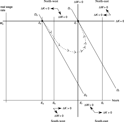
Refer to Figure 2. Assume in the basecase forecast that the economy is perpetually at δ0, that is employment and the real wage rate remain at E0 and W0. Labour supply (people wanting to work) is permanently at S0: we draw the supply curve vertically on the assumption that the wage rate for non-employment is indexed to the wage rate for employment so that movements in the wage rate for employment do not affect the relative attractiveness to workers of employment and non-employment. Unemployment is fixed at S0 minus E0. At this level of unemployment we assume that there is no pressure from the labour market to change the real wage rate.
Dynamic Adjustment of Employment and Wages Under a Labour-market Program
We specify the labour demand function as
E t = Kt * g(Wt)
(11)where:
E t is employment in year t;
K t is the capital stock; and g is a decreasing function of the real wage rate, Wt.
In Figure 2, the year-0 labour-demand curve is D0D0.
We assume that the rate of return on capital at δ0 is equal to the exogenously given world rate, so that there is no tendency for K to change from K0 or for the demand curve for labour to move.
For the policy run we assume that a labour-market program is implemented that moves the aggregate supply of labour in year 0 from S0 to Sf. With this new level of supply, the employment level at which the rate of unemployment is the same as the initial rate is Ef, where Ef satisfies
E 0/S0= Ef /Sf.
(12)Given the shift in supply from S0 to Sf, how will the economy evolve from its initial employment–wage point, δ0? To answer this question, we consider the behaviour of the real wage rate (W) and the capital stock (K) in the four quadrants of Figure 2 defined by the horizontal line through W0 and the vertical line through Ef.
(ii) The Dynamic Path of the Employment–Wage Point Wage Behaviour (Movement along the Labour-demand Curve)
Simplified so that it can be used in the context of Figure 2, the MONASH wage-adjustment specification (8), is:
 (13)
(13)In the policy run,
S t =Sf for all t.
(14)Consequently, the wage rate will be decreasing from year to year in the policy run whenever
 (15)
(15)that is
ΔW < 0 whenever Et < Ef .
(16)In terms of Figure 2, the real wage rate falls in the north-west and south-west quadrants. Similarly, it rises in the north-east and south-east quadrants. It is stationary on the vertical line through Ef. At any given level of capital stock (i.e. at any given position of the labour-demand curve), labour-market pressures move the employment–wage point along the labour-demand curve. This is indicated in Figure 2 by the direction of the ΔW-arrows.
Capital-stock Behaviour (Movement of the Labour-demand Curve)
We assume that the rate of return (Rt) on an additional unit of investment at time t is an increasing function of the marginal product of capital, which in turn is a decreasing function of the ratio of capital input (Kt) to labour input (Et). Hence,
 (17)
(17)where h is a decreasing function.
Next, we assume that the real wage rate in t(Wt) equals the marginal product of labour (MPL), that is
 (18)
(18)where MPL is an increasing function of Kt/Et.
If Rt is greater than the initial rate of return, R0, then there will be capital inflow, causing the capital stock to increase and the labour-demand curve to move rightward.
We can conclude from (17) and (18)

Thus, the labour-demand curve moves to the right whenever Wt < W0.
In terms of Figure 2, the labour-demand curve moves right in the south-west and south-east quadrants. Similarly, it moves left in the north-west and north-east quadrants. It is stationary on the horizontal line through W0. These capital-market pressures are indicated in Figure 2 by the direction of the ΔK-arrows.
Dynamic Path
Starting fromδ0, the employment–wage point δt will be forced initially by labour-market pressures to move down D0D0 into the south-west quadrant of Figure 2. In this quadrant, labour- and capital-market pressures combine to move δt south-easterly until it reaches the vertical boundary through Εf. At this stage, δt must pass into the south-east quadrant on a path with zero slope.
In the south-east quadrant, δt initially moves north-easterly. Eventually, δt must leave the south-east quadrant by arriving at the horizontal boundary through W0. It cannot leave by crossing back into the south-west quadrant: if δt approached the vertical boundary through Ef, then wage pressures would be negligible (ΔW= 0) and δt would be pushed back into the south-east quadrant by capital pressures (ΔΚ > 0).
There are two possibilities for δt's departure from the south-east quadrant. The first is that δt arrives directly at the new steady-state equilibrium, δf. This possibility is shown by the dotted line in Figure 2. The second possibility is that the labour-demand curve overshoots its steady-state position. In this case, δt would cross into the north-east quadrant. It would then travel north-westerly and cross into the north-west quadrant from whence it would travel back into the south-west quadrant. In a sensibly parameterised model, δt would eventually arrive at δf from the south-east quadrant via a converging spiral.
(iii) Behaviour of the Displacement Percentage
Assume that the population is made up of two groups, i = 1, 2. Supply of labour from i at time t is Lit and total supply is
S t =L1t+L2t.
(19)Assuming that each supplying worker has an equal chance of getting a job, employment of the two groups is
E it =Ait * Et
(20)where
 (21)
(21)Assume that basecase supply and employment for both groups are fixed at their initial values, L10, L20, E10 and E20. In the policy run, we introduce a labour-market program targeted on group-1 non-employed people. Assume that the program causes a one-off increase in labour supply from group 1 but does not affect supply from group 2. In terms of Figure 2, all of the shift in supply from S0 to Sf is accounted for by a shift in supply from group 1. What happens to the displacement percentage, D(t), in the transition from δ0 to δf?
To answer this question, we start by re- interpreting −ΔJt in (1) as the deviation caused by the program in the number of group-1 people who obtain jobs (this is legitimate here because the target group is all group-1 non-employed). Next, we divide the numerator and denominator of (1) by E0 to obtain
 (22)
(22)where e1t and et are the program-induced percentage deviations at time t in employment of group 1 and total employment, and A10 is the basecase share of group i in total employment (and labour supply).
With supply from group 2 fixed (l2t= 0), percentage–deviation forms of (19), (20) and (21)8 give
A 10 * e1t=A20 * st+ A10 * et
(23)where lowercase symbols refer to program-induced percentage deviations in the variables denoted by corresponding uppercase symbols. Using (23) to eliminate e1t from (22), we obtain
 (24)
(24)Formula (24) reveals the following:
- •
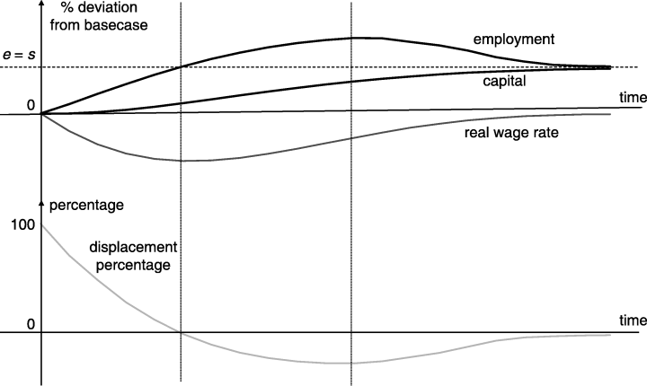
If et is zero, then displacement is 100 per cent. Hence, displacement will be high in the early years of a labour-market program. In terms of Figure 2, displacement is high when we first move away from δ0.
- •
Displacement falls towards zero as et approaches st. This means displacement declines from 100 per cent towards zero as δt moves south-east through the south-west quadrant.
- •
Displacement is zero when et=st. Thus, displacement reaches zero when δt reaches the vertical boundary through Ef. Equivalently, displacement is zero when the deviation in the real wage reaches its largest negative percentage value.
- •
Displacement is negative when et is greater than st, implying that displacement becomes negative when δt crosses into the south-east quadrant. If δt moves directly to δf (as illustrated in Figure 2), then displacement will converge to zero from below. If δt moves to δf along a converging spiral, then displacement will asymptote to zero with damped oscillations.
The stylized model described here sets up expectations concerning results from MONASH for the effects of labour-market programs. These expectations are summarised in Figure 3. In this figure, we follow the dotted path in Figure 2 and draw the deviation paths for employment, capital and the real wage, together with the implied path for the displacement percentage. Where MONASH results differ from those expected on the basis of the stylised model, we need to look for and assess the mechanisms in MONASH that cause the differences.
Effects of a Labour-market Program in a Stylised Model
IV Effects of Two Types of Labour Market Programs: Results from MONASH
(i) Simulation 1: Provision of Job Information
The status of the target group in this simulation is long-term non-employment, defined broadly to include discouraged workers and covering about 9 per cent of the potential work force. For the characteristic of the target group, we arbitrarily choose left-handedness to emphasise that the characteristic is unobserved or irrelevant to employers. The target group (long-term non-employed left-handers) can provide inexperienced labour services that are identical to those of other suppliers of these services. In all years of our basecase, we assume that the proportion of left-handers is 10 per cent in each of the W, N, SE, SI and LN categories. Thus, our target group comprises about 0.9 per cent of the potential labour force.
In the policy run, we introduce a job-information program that encourages target people to apply for jobs by causing a shift in their preferences towards work activities. We represent these preference shifts as 5 per cent shocks in 2007 to a subset of the Bq,v,t's appearing in the utility function (5). The shocks are administered in the policy run via (7) with the inclusion among the shocks for 2007 of:
b q,v= 5 for q equals target group and for all employment activities v. (25)
MONASH results generated under (25) are shown in 4-7. With the exception of the displacement percentage in Figure 5, all results are expressed as percentage deviations between variable values in the policy and basecase runs.9

Macro Variables: Information Program (Percentage Deviations from Basecase)

Displacement Percentage: Information Program
Real Before-tax Wage Rates: Information Program (Percentage Deviations from Basecase)
Real After-tax Wage Rates: Information Program (Percentage Deviations from Basecase)
The results in 4, 5 are highly compatible with those from our stylised model (compare with Figure 3). The main differences concern the displacement percentage. In Figure 5:
- 1
The displacement percentage passes through zero after the real wage rate troughs rather than at the same time, or equivalently, the displacement percentage is positive when the wage rate troughs rather than zero.
- 2
The displacement percentage asymptotes in the long run above zero rather than at zero. What are the features of MONASH that cause these differences?
Why is the Displacement Percentage Positive When the Real before-tax Wage Rate Troughs?
In the stylised model, we assumed that the supply of labour to employment is completely exogenous (the supply curves in Figure 2 are vertical). The labour-market program simply causes an exogenous increase in offers to employment from the target group and no change in the offers from the non-target group. By contrast, in MONASH a labour-market program can affect offers to employment endogenously. It does this by altering wage rates and causing changes in offers to employment not only by people in the target group but also by people outside that group.
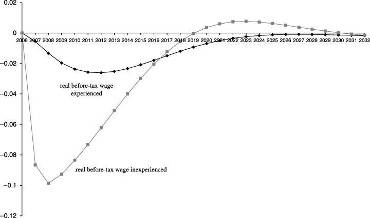
As can be seen from Figure 6, under the provision-of-information policy, shock (25), there is an immediate reduction in the real before-tax wage rate of inexperienced workers relative to that of experienced workers. This reflects the initial increase in the supply of inexperienced labour from the left-handed long-term non-employed. In terms of (8), shock (25) causes an immediate increase in  for all oe where oe is an inexperienced work activity.
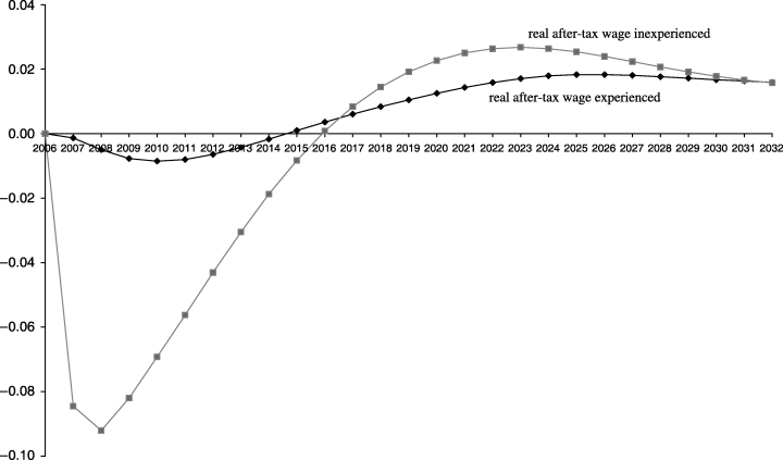
The change in the relative real before-tax wage rates translates into a similar change in relative after-tax wage rates (Figure 7). With a decrease in inexperienced after-tax wage rates relative to experienced after-tax wage rates, the benefit for non-employment increases relative to the inexperienced after-tax wage rate. This is because we assume that the benefit rate moves with the average after-tax wage rate [see (10)]. The increase in the benefit rate relative to the wage rate for inexperienced employment causes a reduction in offers to employment by non-target people who can offer inexperienced labour (particularly categories SI1, SI2 and LN2, see Figure 1). This means that the overall increased level of supply to employment is comprised of an increase in supply by the target group and a partially offsetting decrease in supply by the non-target group.
Thus, in the policy simulation, at the point of no wage pressure when the percentage increase in supply is matched by the percentage increase in employment, there is a positive deviation in employment of the target group and a negative deviation in employment of the non-target group.10 Consequently, at this point (when the wage rate troughs), the displacement percentage is positive.
Why does the Displacement Percentage Asymptote above Zero in the Long Run?
The information program has a long-run positive effect on aggregate employment, thereby increasing the aggregate supply of experienced workers. Despite reducing the number of long-term non-employed workers, the program has a positive effect on aggregate supply of inexperienced labour: the increase in supply per left-handed long-term non-employed person happens to more than offset the decrease in the number of long-term non-employed people. It happens in the long run that the percentage increases in the supplies of inexperienced and experienced labour are approximately matched. Thus, as can be seen from 6, 7, the long-run deviations in the wage rates (in either before- or after-tax terms) of experienced and inexperienced workers are approximately the same.11
This means that there are no long-run incentives for non-target people to shift their offers between employment and non-employment activities. So why is the displacement percentage positive in the long run, implying a negative deviation in employment of non-target people?
The answer is that the program causes a long-run positive deviation in the number of people in short-run experienced non-employment: this category of non-employment is fed mainly by severances and severances are modelled as an almost fixed share of employment meaning that they rise with aggregate employment. As short-run experienced non-employment is a non-target category of non-employment, its increase explains the small long-run positive displacement percentage that can be seen in Figure 5.
(ii) Simulation 2: Reducing benefits to A Subset of the Non-employed
This time, the program is a 5 per cent reduction in the benefits to the long-term non-employed left-handers introduced in 2007 in the policy run by setting:
f q,g = −5 for q equals target group and g equals the activity long-term unemployment,
(26)where fq,g is the percentage deviation in Fq,g,t appearing in (10).
MONASH results generated under (26) are shown in 8-11. Again, the main differences between the MONASH and stylised results concern the displacement percentage. This time the displacement percentage in the MONASH results asymptotes in the long run below zero rather than at zero.
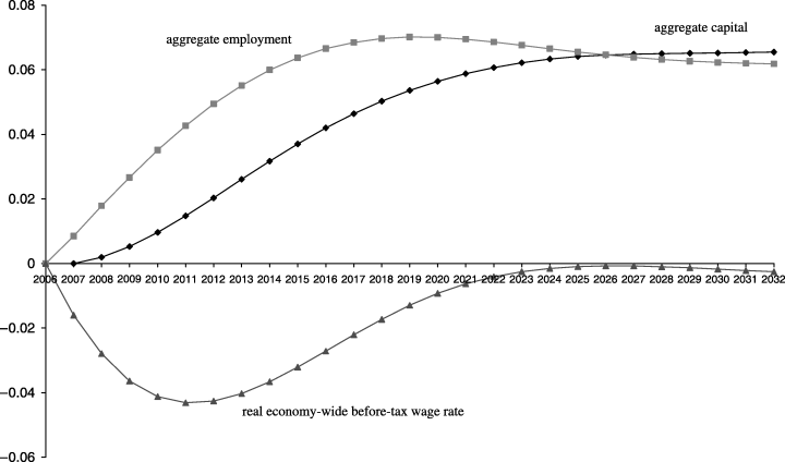
Macro Variables: Benefit-cut Program (Percentage Deviations from Basecase)
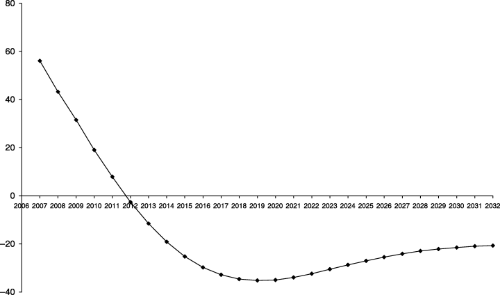
Displacement Percentage: Benefit-cut Program

Real Before-tax Wage Rates: Benefit-cut Program (Percentage Deviations from Basecase)

Real After-tax Wage Rates: Benefit-cut Program (Percentage Deviations from Basecase)
The programs in both MONASH simulations work primarily through an outward shift in the supply-to-work curve of left-handed long-term non-employed people. However, the benefit-cut program has two additional effects. First, it directly changes the supply incentives of left-handed short-term non-employed people. It induces them to increase their offers to employment and reduce their offers to non-employment (where they would receive a reduced benefit). Second, as can be seen from Figure 11, the benefit-cut program causes a long-run increase in the real after-tax wage rate of inexperienced workers relative to experienced workers. This causes a further reduction in the benefit : wage ratio for all non-employed people who could potentially offer inexperienced labour. Thus, in the long run, the benefit-cut program causes an increase in offers to employment and ultimately an increase in employment of people in non-target non-employment categories. Consequently, the increase in aggregate employment exceeds the increase in employment of target people, explaining the negative long-run displacement percentage.
But why does the benefit-cut program cause a long-run increase in the real after-tax wage rate of inexperienced workers relative to experienced workers whereas this was not the case in the information program (compare 11, 7)? The answer lies mainly in the supply response of short-term experienced, non-employed left-handers (SE1). In the benefit-cut program, but not in the information program, these people increase their supply of offers to experienced employment. This increases the inexperienced/experienced wage ratio in the benefit-cut program.
V Concluding Remarks
A key question concerning any labour-market program is the extent to which it generates jobs for the target group at the expense of other groups. This effect is measured by the displacement percentage. Simple economic theory suggests that displacement percentages are high in the short run and zero in the long run.
In the stylised model in Section III, a labour-market program initially increases the share of the target group in offers to fill job vacancies without affecting the number of vacancies. This enables the target group to increase its share in successful applications for jobs. Thus, in the short run, target-group employment increases, whereas non-target-group employment falls. In the longer term, increased overall offers to employment (increased overall labour supply) relative to the number of vacancies puts downward pressure on real wage rates. Slower growth in real wage rates allows faster growth in employment both through movement down labour-demand curves and through increased profitability with consequent expansion of capital and outward shifts in labour-demand curves. As expansion in aggregate employment continues, the displacement percentage falls to zero, and may temporarily become negative, but eventually return to zero.
In Section IV, we reported results from MONASH on the effects of two types of labour-market programs: information provision and benefit cuts. Our results were broadly consistent with the simple theory described in Section III. We found that:
- 1
active labour-market programs can generate significant long-run increases in aggregate employment; and
- 2
short-run displacement percentages are much larger than long-run displacement percentages.
However, our detailed modelling revealed that displacement percentages are quite sensitive to the nature of a labour-market program. An insight from the modelling is that incentive effects for non-target groups are important in determining displacement. For example, we found that a benefit-cut program applied to a target group of long-term non-employed people may discourage non-target people from entering long-term non-employment. This leads to negative long-run displacement effects.


