Non-stationarity and local approaches to modelling the distributions of wildlife
ABSTRACT
Despite a growing interest in species distribution modelling, relatively little attention has been paid to spatial autocorrelation and non-stationarity. Both spatial autocorrelation (the tendency for adjacent locations to be more similar than distant ones) and non-stationarity (the variation in modelled relationships over space) are likely to be common properties of ecological systems. This paper focuses on non-stationarity and uses two local techniques, geographically weighted regression (GWR) and varying coefficient modelling (VCM), to assess its impact on model predictions. We extend two published studies, one on the presence–absence of calandra larks in Spain and the other on bird species richness in Britain, to compare GWR and VCM with the more usual global generalized linear modelling (GLM) and generalized additive modelling (GAM). For the calandra lark data, GWR and VCM produced better-fitting models than GLM or GAM. VCM in particular gave significantly reduced spatial autocorrelation in the model residuals. GWR showed that individual predictors became stationary at different spatial scales, indicating that distributions are influenced by ecological processes operating over multiple scales. VCM was able to predict occurrence accurately on independent data from the same geographical area as the training data but not beyond, whereas the GAM produced good results on all areas. Individual predictions from the local methods often differed substantially from the global models. For the species richness data, VCM and GWR produced far better predictions than ordinary regression. Our analyses suggest that modellers interpolating data to produce maps for practical actions (e.g. conservation) should consider local methods, whereas they should not be used for extrapolation to new areas. We argue that local methods are complementary to global methods, revealing details of habitat associations and data properties which global methods average out and miss.
INTRODUCTION
Interest in building models to predict the distributions of organisms is increasingly popular in applied ecology. General and specific reviews (e.g. Guisan & Zimmerman, 2000; Scott et al., 2002; Gottschalk et al., 2005; Pettorelli et al., 2005), special issues of journals (e.g. Ecological Modelling 2002; Biodiversity and Conservation 2002; Journal of Applied Ecology 2004, this issue of Diversity and Distributions), and international meetings (e.g. Riederalp, Switzerland 2001, 2004; Baeza, Spain, 2005) all attest to the activity of researchers in this field. Progress has been made in laying the ecological foundation for predictive distribution modelling (Austin, 2002) and models have been built to understand niche requirements, for nature conservation, to predict the impacts of land use or environmental change on a species, and to assess the risks of biological invasions. A wide range of techniques (Segurado & Araujo, 2004) has been applied to organisms such as invertebrates, fish, amphibians, lower and higher plants, birds, and mammals.
Application of new techniques and to new situations has outstripped attention to issues of data quality, spatial scale, and meeting the assumptions of the techniques applied. Two issues stand out, spatial autocorrelation and stationarity, both of which interact with spatial scale. Spatial autocorrelation is the tendency for objects that are close together to be more similar than those that are further apart and is a widespread and natural property of ecological systems (Legendre, 1993). Nonetheless, until recently (e.g. Segurado & Araujo, 2004; Luoto et al., 2005) most published distribution studies have ignored spatial autocorrelation despite the availability of methods to incorporate it within the familiar GLM context (Legendre, 1993; Augustin et al., 1996). The second spatial issue, stationarity, has received even less attention from distribution modellers (e.g. in a recent evaluation of modelling approaches, Segurado & Araujo (2004) considered spatial autocorrelation but not stationarity). In contrast to spatial autocorrelation, stationarity is a property of the modelled relationship rather than the data. A process is called stationary if the statistics that define it and measured within any subset accurately describe the statistics of the entire data. Stationarity here therefore refers to the tendency for any relationship or process being modelled (e.g. a plant's response to pH or the food preferences of an animal) to vary spatially. Interregional differences in modelled relationships can arise through models not being fully specified, because habitat availability differs spatially, and, more interestingly, because widespread species often show variation in ecological characteristics across their ranges. For example, golden eagles Aquila chrysaetos show different habitat associations among study sites in Scotland despite similar proportions of habitat being available (Fielding & Howarth, 1995). Importantly, spatial models may need to account for autocorrelation, non-stationarity, and their interaction, i.e. that the tendency for neighbouring pixels to be more similar than distant ones (autocorrelation) varies spatially (non-stationarity). What most distribution modelling studies have in common is the desire to build a global model capable of accurately predicting the occurrence of a species or group of species. By ‘global’ we mean a model that is equally effective at any location. The critical issue for distribution modellers using commonly employed regression methods is that regression coefficients cannot be assumed to be constant for non-stationary relationships. In fact, global regression models may even mask the processes being studied because they give an average picture of the relationships between the predictor and the response variables. The danger is that the averaged relationship, although amenable to elegant description by response curves and interpretation through ecological theory, may in fact never exist in nature. The purpose of this paper is therefore to explore how distribution models might take into account spatial non-stationarity and to illustrate its impacts on model predictions. The focus here is on prediction success since this is the goal of most distribution modelling studies but far more needs to be done on interpreting models that explore stationarity.
If regression coefficients cannot be assumed to be constant over space (i.e. global), methods that allow them to vary locally are needed. Assunção (2002) provides a useful brief review of approaches to studying spatial stationarity using a variety of space-varying coefficient models. Here we focus on two methods: geographically weighted regression (GWR) (Brunsdon et al., 1998), and varying coefficient modelling (VCM) (Hastie & Tibshirani, 1993). Osborne & Suárez-Seoane (2002) pointed out how partitioning data geographically can improve the fit of distribution models and suggested that GWR, as the logical extension of data partitioning, might offer a solution. Foody (2004, 2005) has applied the technique to predictive models of species richness, while Wang et al. (2005) and Zhang et al. (2004, 2005) have used it in other ecological contexts. GWR calculates a regression solution for each location or data point in the data set. It does this either by defining a distance (bandwidth) within which surrounding observations are included in the analysis, or by using an adaptive kernel that alters the inclusion distance to encompass a defined number of data points. Observations are weighted as a function of their distance from the location being predicted. GWR is thus a geographically local regression method where data points contribute in a manner that is weighted positively by their proximity to the location under study. Varying coefficient models, in the context here, are a class of local models where the regression coefficients of generalized linear models vary as smooth functions of location (Hastie & Tibshirani, 1993). Such models retain the familiar GLM structure but subject the regression coefficients to ‘effects modifiers’ which change their values across space. VCM may be carried out by specifying a GLM with a full interaction with easting and northing using natural smoothing splines (T. Hastie, pers. comm.).
In this paper we extend two existing studies to explore the assumption of stationarity in distribution models. From the first, a comparison of three cereal steppe birds in Spain (Suárez-Seoane et al., 2002), we arbitrarily choose one species (the calandra lark Melanocorhypha calandra) as typical of many recent studies on the presence–absence distributions of animals and plants. The calandra lark is a small songbird occupying open cereal and steppe-like habitats and its distribution in Spain has been modelled successfully using generalized additive modelling (Suárez-Seoane et al., 2002). Our aim here was to discover whether non-stationarity existed in the data set and to assess what impact it had on model predictions. The second study (Foody, 2005) looked at bird species richness in Great Britain, rather than the presence or absence of a single species. Here we extend Foody's (2005) analysis to compare the performance of GWR and VCM for predicting species richness against his global regression model. Our working hypothesis for both data sets was that the space-varying modelling approaches would outperform global models by capturing local variation and so produce more accurate predictive distribution maps.
METHODS
The calandra lark data set, its predictor variables, and baseline GAM model are described in detail by Suárez-Seoane et al. (2002). The bird data comprised 2900 presence and confirmed absence records in equal numbers gathered on a 1-km2 grid from across Spain during 1993–2001. As a first stage in analysis, we re-generated the GAM of Suárez-Seoane et al. (2002) by modelling the bird data against predictors for green biomass, linear features such as roads and rivers, urban developments, and altitude and terrain variability using a logit link with binomial error structure. By examining the response curves for variables with significantly nonlinear relationships, we determined that a quadratic term could adequately approximate the splines and thus specified a polynomial GLM to mimic the GAM. Note that polynomial GLMs can rarely duplicate GAMs precisely and our aim was to find an adequate rather than equivalent nonlinear model. The linear and squared terms in the polynomial GLM were then used in a logistic GWR to generate the GWR solution. We used a Gaussian kernel of fixed bandwidth (100, 200, and 250 km on different runs) to specify the search radius and weighting for inclusion of neighbouring data points. As GWR generates a regression coefficient for each variable at each data point, it is possible to use the variation in the coefficients as an approximate index of stationarity (Brunsdon et al., 1998). For each variable, we calculated the interquartile range in the GWR coefficient and divided it by two times the standard error of the global regression coefficient for the same variable from the GLM. Recalling that about 68% of the data lies within one standard deviation and 50% between the quartiles, the ratio of the two provides an approximate measure of stationarity where values greater than one indicate non-stationary (Charlton et al., 2003). We plotted the change in this index against the bandwidth to determine at what spatial scale the relationship between the response and the predictor variable became stationary. GWR calculations were performed using the gwr 3.0 software available at http://ncg.nuim.i.e./ncg/GWR/. The VCM was specified as a full interaction of the polynomial GLM with the natural splines of latitude and longitude within a Generalized Additive Model in s-plus (Hastie & Tibshirani, 1990). These analyses provided comparable predictive models for the calandra lark over the whole of Spain.
The aspatial fit of the models was assessed using the nonparametric area under the receiver operating characteristics curve (AUC) (Beck & Shultz, 1986) and spatial pattern in the fit through analysis of residuals. Model residuals were defined as the difference between the observed and predicted values, and their spatial distribution was investigated using global and local Moran coefficients (Anselin, 1995; Zhang et al., 2005). The global Moran coefficient is positive when the residuals at neighbouring locations are similar, negative when they are dissimilar, and approximately zero when no spatial autocorrelation exists. We defined the neighbourhood distance as 50 km (approximately the minimum possible on our data set) and 100 km (to correspond with the optimum bandwidth of the GWR). Significance was assessed through a random permutation test using 999 runs (Anselin, 2003). Global Moran coefficients may be decomposed to assess spatial autocorrelation around each data point, a process termed Local Indicators of Spatial Association or LISA (Anselin, 1995). Maps of local Moran coefficients identify clusters of residuals that deviate from the mean and provide a valuable tool for locating hotspots on maps (Boots, 2002; Dale & Fortin, 2002). Analysis of residuals was performed using the geoda version 0.9.5 software (Anselin, 2003).
We next divided the data set into three to test different facets of model fitting and predictive performance. First, we located a square of 250 × 250 km in the centre of Spain (Fig. 1). Its location was arbitrary except that we wished to keep it away from the spatial boundaries of the total data set and tried to encompass a good sample size and spread of data points. We randomly divided the data within the central square into a training (80%) and a test (20%) data set. All data points outside the central square became a second test set (sample sizes in Table 1). This arrangement allowed us to test predictive performance on a geographically identical data set and one that was immediately adjacent but beyond the geographical range of the training set. We applied the GAM, GLM, and VCM approaches as above to the training data set from the central square and used the resultant models to make predictions on the test sets from the same square and from outside. Note that making predictions beyond the spatial domain of the data is computationally impossible with GWR and only logical with VCM if broad-scale trends are assumed in the fit of the global GLM (which drives the VCM) and coordinate space.
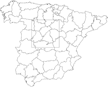
Location of the central sampling area (250 km × 250 km) in Spain used for building and testing models for calandra lark occurrence.
| Training set (within central area) | Test set (within central area) | Test set (outside central area) | Entire data set | |
|---|---|---|---|---|
| GAM | 0.869 ± 0.013 | 0.883 ± 0.023 | 0.907 ± 0.007 | 0.896 ± 0.006 |
| GLM | 0.856 ± 0.013 | 0.878 ± 0.024 | 0.899 ± 0.007 | 0.886 ± 0.006 |
| VCM | 0.916 ± 0.010 | 0.934 ± 0.017 | 0.953 ± 0.004 | 0.943 ± 0.004 |
| GWR (100-km bandwidth) | 0.903 ± 0.011 | 0.926 ± 0.017 | 0.941 ± 0.005 | 0.930 ± 0.005 |
| Sample size | 820 | 204 | 1876 | 2900 |
The fit of the models and their predictive performance on independent data was again assessed using the area under the AUC. Comparison of performance among competing models was achieved using the correlated area test statistic that assesses the significance of differences in AUC scores (software package rockit at http://www-radiology.uchicago.edu/krl/KRL_ROC/software_index.htm). The probability indices (habitat suitability scores) generated by each modelling approach were compared directly using rank correlation analysis. Finally, the predictive maps produced were compared using the method of Pontius (2000) which partitions Kappa into separate indices for location and quantity errors. To achieve this, the probability scale on each map was re-classed into 10 equal intervals to create categorical maps and the GLM map specified as the reference map for comparison.
The species richness data set came from Gibbons et al. (1993) and comprised the presence–absence records of 199 bird species in 2578 squares of 10 × 10 km in Great Britain. Foody (2005) has previously shown how these data may be modelled using GWR and here we extended the analysis to include the VCM approach and compare the mapped predictions. The GWR was run with a fixed bandwidth of 50 km using a Gaussian kernel. We used conventional ordinary least squares (OLS) regression on these data because trials with Poisson family models gave very similar results and no advantages (also see Discussion for consideration of nonlinear relationships). Model fit was assessed using r2 and maps compared with the method of Pontius (2000), specifying the true richness map as the reference image and re-classing each map into eight categories.
RESULTS
Models for the calandra lark across the whole of Spain
The fit of the models applied to the whole of Spain was better in terms of AUC for the GAM than the GLM, and better again for the spatially varying GWR and VCM (Table 1). Comparison of the predictions arising from the models showed that the GLM and GAM were tightly correlated, the GWR and VCM less so, but both spatially varying approaches made significant changes to the predictions from the GLM (Fig. 2). Some shifts exceeded 0.5 (on a 0–1 scale) and would be classed as different even on an ‘honest’ probability scale (i.e. one avoiding spurious accuracy — see Hirzel et al., in press).
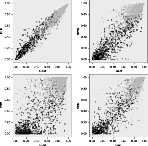
Comparison of the probability scores obtained from four different approaches to modelling the presence–absence of calandra larks across the whole of Spain: GLM, generalized linear modelling; GAM, generalized additive modelling; VCM, varying coefficient modelling; GWR, geographically weighted regression (bandwidth at 100 km). The grey points are true presence and the black points true absence.
The improvement in the fit of the GWR over the GLM was scale dependent (Table 2), peaking at 100-km bandwidth (smaller bandwidths could not be tested for technical reasons). Note, however, that predictor variables became stationary at different bandwidths (Fig. 3), perhaps indicating that the ecological processes that affect distributions operate at different spatial scales. For example, while the vegetation component PC5 appeared to become stationary somewhere between the 150 m and 200 m bandwidths, the vegetation component PC1 did not become stationary within the range of bandwidths tested.
| Model | GWR bandwidth | Corrected AIC | AUC ± SE |
|---|---|---|---|
| GWR | 100 km | 2159.72 | 0.930 ± 0.005 |
| GWR | 200 km | 2314.49 | 0.905 ± 0.006 |
| GWR | 250 km | 2350.59 | 0.899 ± 0.006 |
| GLM | — | 2441.24 | 0.886 ± 0.006 |
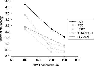
Index of stationarity for five of the predictor variables used in the geographically weighted regression models for the occurrence of calandra larks in Spain (chosen to illustrate a range of responses). The index is the interquartile range in a regression coefficient from a geographically weighted regression compared with twice its standard error from a comparable but spatially constant model. Values above 1 are indicative of non-stationarity at the spatial scale (bandwidth) shown. The variables PC1, PC5, and PC12 are components of vegetation, TOWNDIST is the distance to the nearest town, and RIVDEN is the density of rivers within a 1 km2 pixel.
Analysis of the residuals from the four models showed the presence of significant spatial autocorrelation in all but the VCM approach within 50-km and 100-km neighbourhoods. Global Moran's I was similar for the GAM and its GLM mimic, substantially less for GWR and close to zero for VCM (Table 3). All significant values of Moran's I were positive, indicating clustering of residuals with similar values (i.e. consistent local deviation from a global relationship). Spatial autocorrelation was less apparent with a 100-km than a 50-km neighbourhood for all approaches where Moran's I was significant.
| 50-km neighbourhood | 100-km neighbourhood | |||
|---|---|---|---|---|
| Global I | Significance | Global I | Significance | |
| GAM | 0.0863 | 0.001 | 0.0460 | 0.001 |
| GLM | 0.0926 | 0.001 | 0.0484 | 0.001 |
| VCM | −0.0008 | 0.449 | 0.0004 | 0.298 |
| GWR (100-km bandwidth) | 0.0295 | 0.001 | 0.0100 | 0.001 |
Although the VCM reduced the residual spatial autocorrelation to levels of non-significance at the global scale, pockets of deviant residuals remained and were detectable using LISA (Table 4; Fig. 4). Nevertheless, VCM (as the best local modelling approach) showed approximately three to 11 times fewer locations with significant local autocorrelation than the best global modelling approach (GAM), depending on significance level and neighbourhood distance. The central part of the study area was apparently difficult to model (cf. 1, 4) and this would explain why the fit of the national-scale models when partitioned into the three areas used in the next section was best outside the central area (Table 1). Most values for local Moran's I were positive, indicating clusters of data points with similar values that deviated strongly (either positively or negatively) from the mean (see Zhang et al., 2005).
| % significant at P < 0.05 | % significant at P < 0.01 | % positive | % negative | ||
|---|---|---|---|---|---|
| 50-km neighbourhood | GAM | 62.3 | 45.8 | 62.0 | 38.0 |
| VCM | 16.4 | 6.2 | 57.8 | 42.2 | |
| 100-km neighbourhood | GAM | 80.6 | 67.7 | 55.8 | 44.2 |
| VCM | 14.0 | 6.0 | 60.4 | 39.6 | |

Plots in geographical space of the significance of local Moran's I coefficients for the varying coefficient modelling (top row) and generalized additive modelling (bottom row) approaches at two neighbourhood distances. The plots show locations where local I was significant at the 0.05 level and circle size is proportional to significance from 0.05 (smallest circles) to 0.002 (largest circles). The area of each plot corresponds to the whole of Spain as in Fig. 1. Sample size in each case was 2900 locations.
Partitioned models for the calandra lark
The partitioned models were built on the training data set from the central area and then applied to test data sets both within and outside the area (Table 5). As with the national scale models, the GAM fitted the training data better than the GLM but both were outperformed by the VCM. As expected, these locally applied models were better than the partitioned results from the national models for all modelling techniques (compare AUC values in Tables 1 and 5). When applied to the test data, however, the VCM performed well on data from within the same geographical area but was no better than a random model outside it. In contrast, the GAM and to a lesser extent the GLM performed tolerably well on both test data sets. Results of AUC comparisons show that the VCM did not produce significantly better predictions than the GLM or the GAM on the test data set within the same geographical area (Table 6), although this may have been due to the smaller sample size of the test data set (20%). Predictions outside the same geographical area were significantly worse for the VCM than either the GLM or the GAM (Table 6).
| Training set (within central area) | Test set (within central area) | Test set (outside central area) | |
|---|---|---|---|
| GAM | 0.891 ± 0.011 | 0.880 ± 0.024 | 0.823 ± 0.010 |
| GLM | 0.871 ± 0.012 | 0.883 ± 0.023 | 0.794 ± 0.011 |
| VCM | 0.946 ± 0.008 | 0.903 ± 0.021 | 0.511 ± 0.013 |
| Training set (within central area) | Test set (within central area) | Test set (outside central area) | |
|---|---|---|---|
| GAM vs. GLM | 4.721, P < 0.001 | 0.732, ns | 3.046, P = 0.002 |
| GAM vs. VCM | 6.393, P < 0.001 | 1.278, ns | 14.746, P < 0.001 |
| GLM vs. VCM | 7.799, P < 0.001 | 0.697, ns | 14.629, P < 0.001 |
Comparison of the VCM and the GLM showed that even on the training data set there was a measurable disagreement between the models (Spearman's rank correlation, r = 0.83; Table 7). The VCM tended to produce more extreme values that could be regarded either as better discrimination of presence and absence points or as over-fitting of the data. However, tests for over-fitting (Vaughan & Ormerod, 2005) showed that this was not a problem (Fig. 5). Partitioning of Kappa confirmed that the GLM- and the GAM-predicted maps (Fig. 6) were more similar than the GLM and VCM maps (Kno = 0.513 and 0.274, respectively, in Table 8). The VCM map differed more in both the location of each probability category and especially in the quantity. Despite this, a change to perfect the quantity without changing location (VPIQ) would improve the percentage correctly classified by only 8.6%, whereas perfect location (VPIL) without changing the quantity would improve the accuracy by 37.5% (Table 8).
| Training set (within central area) | Test set (within central area) | Test set (outside central area) | |
|---|---|---|---|
| Sample size | 820 | 204 | 1876 |
| GAM vs. GLM | 0.94 | 0.95 | 0.70 |
| GAM vs. VCM | 0.80 | 0.82 | −0.14 |
| GLM vs. VCM | 0.83 | 0.80 | 0.18 |
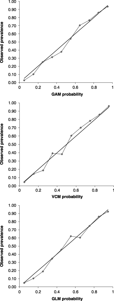
Tests for over-fitting of the predictive models in Fig. 5. A perfect model would follow the leading diagonal and none of the models here shows problems. Note especially that the varying coefficient modelling is no poorer from the generalized linear modelling or the generalized additive modelling. See Vaughan & Ormerod (2005) for further details.
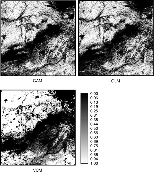
Predictive maps for the occurrence of calandra larks in the central area of Spain shown in Fig. 1 produced by three modelling approaches. Note how varying coefficient modelling produced better discrimination and how some areas (e.g. bottom left corner) are predicted differently by the different models.
| GAM | VCM | |
|---|---|---|
| K no | 0.513 | 0.274 |
| K location | 0.517 | 0.352 |
| K quantity | 0.848 | −0.108 |
| VPIL | 0.410 | 0.375 |
| VPIQ | 0.015 | 0.086 |
Species richness data set
Predictive maps of species richness were generated using a conventional OLS regression model to duplicate Foody (2005), then GWR and VCM (Fig. 7). The explained variance for the GWR (47.1%) and VCM (51.5%) approaches far exceeded that of the OLS model (18.1%). [Note that Foody (2005) reported the r2 for the GWR as 53.9%, the difference arising from improvements to the gwr software between versions 2 and 3 (S. Fotheringham, pers. comm.).] While the GWR and VCM predictive maps were visually very similar, the OLS model falsely predicted a rather even distribution of species across Britain and failed to capture the variation in species richness. Formal map comparison by partitioning Kappa showed that VCM produced the map with the best locational accuracy and quantity within each predicted class (Table 9). GWR performed nearly as well, and both spatially varying techniques were far better than the OLS model.
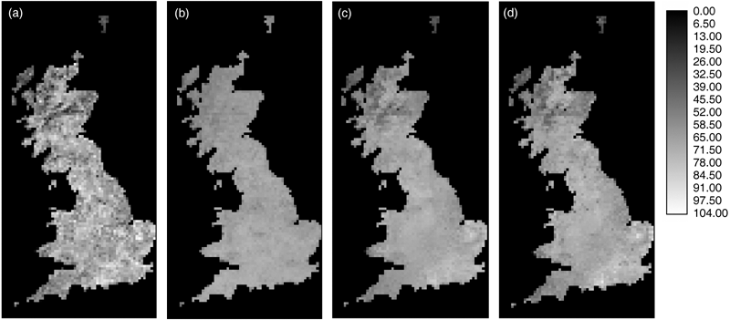
Predictive maps for bird species richness in Britain. (a) raw (actual) data, (b) using ordinary least squares regression, (c) geographically weighted regression, and (d) varying coefficient modelling. The background value has arbitrarily been set to zero.
| OLS | GWR | VCM | |
|---|---|---|---|
| K no | 0.203 | 0.331 | 0.359 |
| K location | 0.097 | 0.312 | 0.314 |
| K quantity | 0.851 | 0.689 | 0.787 |
| VPIL | 0.280 | 0.326 | 0.379 |
| VPIQ | 0.024 | 0.072 | 0.050 |
DISCUSSION
GWR and VCM are local methods that allow regression coefficients to vary over space, removing the assumption of spatial stationarity in distribution modelling. For both the presence–absence data on calandra larks in Spain and the bird species richness data in Britain, these spatially varying methods produced better-fitting models than either the GAMs or the GLMs. Foody's (2005) examination of the species richness data compared only a global OLS approach with the local GWR and could be criticized for not optimizing the global model by considering nonlinear responses. We have retained his models here for comparison with VCM but note that a GAM applied to his data gives r2 = 0.25, better than 0.18 obtained through OLS but considerably less than 0.47 from GWR and 0.52 from VCM.
Little attention has been paid to the spatial patterns in model errors (Zhang et al., 2005), and analysis of residuals provided a powerful way to interpret our models. Global Moran's I differed little between the GAM and its GLM mimic (GAMs were better because they are more flexible) but was noticeably lower for GWR and especially VCM. These local methods achieve success by flexing a model to fit local conditions more closely, although the LISA approach revealed apparent anomalies in the centre of the study area even for VCM. This was coincidentally where we located our sampling area for closer study and the deviant residuals explain why the local fit of our models assessed by AUC to test data was poorer here than elsewhere in Spain.
Local modelling approaches have rarely been used for prediction with presence–absence data, and the software gwr 3.0 (Charlton et al., 2003) lacks the facility to predict on independent data for models with a logit link and binomial error structure. VCM does not suffer this restriction (see also Wheeler & Tiefelsdorf (2005) for other issues on the use of (GWR). We found that VCM gave marginally better predictions than GLM or GAM on independent data within the same geographical area, but was hopeless beyond. This failure beyond the x, y data domain is to be expected since the model has no locational information on which to base the extrapolation. By using adjacent training and test areas, we have shown that this failure can happen immediately after the training data domain is abandoned. On the other hand, a notable advantage of GWR is its facility to identify the spatial scale at which the relationship between the response variable and a predictor becomes stationary. For the Spanish data this differed between predictors and may indicate that the ecological processes influencing distributions operate at different spatial scales. This would suggest that the distribution patterns we see are the result of simultaneous responses to many environmental factors, each acting at different scales.
Despite the success of VCM and GWR, we found that the GAM performed almost as well as the spatially varying methods in terms of aspatial AUC values and was capable of predicting beyond the geographical domain of the data. GLMs are almost as good if built to mimic a GAM once the shapes of the response curves are known. Analysis of residuals, however, revealed the weaknesses in the GAM which VCM partially overcame. These results suggest that modellers should choose their approach carefully according to purpose (see also Segurado & Araujo, 2004). In general, we need to separate models which aim to extrapolate to new areas beyond the geographical range and those which are primarily designed to fill the gaps in existing distributions through interpolation. Locally weighted modelling that relies on geographical coordinates is unlikely to be useful in the former case, but it is highly appropriate in the latter. Thus models predicting shifts in range due to climate change probably cannot make use of geographical information, whereas maps highlighting areas to search for rare species or prioritizing areas for conservation could use geographically weighted modelling to good effect.
While this is a useful general guide on when to use global or local modelling, caution is needed in interpreting any global distribution model ecologically. It has been observed that range size may influence the success of distribution models (McPherson et al., 2004; Segurado & Araujo, 2004) in part because species exhibit variations in habitat associations over large ranges (Stockwell & Peterson, 2002), i.e. the underlying processes are non-stationary. In our data, GWR and VCM improved model performance not by small shifts in probabilities but by reclassifying them across the range from 0 to 1 such that the correlation between the GAM or the GLM with the GWR or VCM was only weak. This confirms our theoretical expectation that because models accounting for non-stationarity are operating on different assumptions than GLMs and GAMs, they are capable of producing quite different results. Direct comparison of predictive maps produced by the space-varying and global methods revealed broad similarities and important differences which could lead to alternative actions (e.g. in the protection of key areas for conservation). Global models sacrifice local fit for generality and the predictive maps and response curves they produce are averages that may mask the underlying environmental processes.
Jetz et al. (2005) commented that if habitat associations are really local, it would be futile to attempt to uncover general relationships through global models. They believe it more likely that relationships are global but appear to vary locally due to missing variables or interactions. We have shown that local modelling approaches can improve even very good global models (in contrast to Foody's (2005) analysis where the global model was weak). Whether habitat associations are global or local is a fundamental ecological issue on which there appears to be little evidence either way. We do not believe that the pursuit of global relationships is futile because individuals of a species should show strong ecological similarities even if there are local variations. Jetz et al. (2005) argue that it is more useful to fit global parameters, allowing for autocorrelation and interactions, than to allow parameters to vary locally using GWR. Our formulation of VCM achieves this by first identifying the global relationship using a GAM and then allowing the model to vary locally through interaction with easting and northing. Analysis of residuals through LISA provides a powerful way to explore spatially how well a model fits the data before and after the global model is flexed locally. We are recognizing the probable general rules for habitat selection or habitat use in a global model and then using an interaction with location to incorporate local variation. Seen in this way, local modelling approaches are not alternatives to global models but complements that allow us to uncover facets of data quality and ecology which generalizations mask, to improve model predictions, and to understand the spatial patterns in model errors.
ACKNOWLEDGEMENTS
We thank John Leathwick, Antoine Guisan, and Peter Atkinson for valuable discussions on spatial autocorrelation and non-stationarity, Stewart Fotheringham for insights into GWR, and Trevor Hastie for ideas on VCM. The British Trust for Ornithology kindly allowed GMF access to the breeding bird data from the 1988–1991 bird atlas. The ideas in this paper were first presented at the workshop ‘Predictive modelling of species distribution. New tools for the XXI century’, organized by the Universidad Internacional de Andalucía, sede Antonio Machado in Baeza, Spain and we thank the organizers for inviting P.E.O. Two anonymous referees and the handling guest editor made valuable comments which improved this paper.


