Nonlinear Effects of Weather on Corn Yields^†

This paper examines the reduced-form relationship between weather and yields using a unique data set of corn yields and daily weather records covering the eastern United States for 1950–2004. Since weather variations in a fixed location are exogenous and random, the reduced-form relationship constitutes a viable natural experiment and is therefore clearly identified. Understanding the precise link between heat and crop yields could have implications for the effects of climate change on food supply. It may also facilitate the creation of financial instruments that may be used to insure crop yield risk without inducing moral hazard.

Previous studies examining the link between weather and yields either used broad aggregate weather measures in a reduced-form regression, or detailed nonlinear weather interactions in a crop-simulation model, where several parameters are set by the researcher and not estimated because of data limitations. This paper provides two key contributions to the literature. First, we compile a unique data set of daily weather records and combine it with a fifty-five-year record of corn yields from almost 2,000 U.S. counties to estimate the relationship between weather and yields. Our data set is unique because it estimates weather outcomes at the specific locations in each county where crops are grown and then calculates the time a crop is exposed to each 1°C temperature interval during a day. Second, these data are detailed enough to allow for a very flexible functional form to accurately estimate nonlinear impacts of weather on yields. We are thus able to precisely estimate nonlinearities in the effect of weather on yields.

Our approach combines the strengths of the reduced-form approach with those of crop-simulation models. The reduced-form natural experiment may be superior to a controlled experiment because we wish to ascertain the consummate effects of weather on yields, which may differ from the effects of weather ceteris paribus. For example, Deschenes and Greenstone find input responses to weather fluctuations by regressing average profits and expenditures in each county from three Census years on average monthly temperatures in four months of the year, including county-fixed effects. The pervasive problem in this literature is the way in which weather variables are measured and the limited flexibility this imposes on the statistical models used to link weather with crop yields. The weather regressors are mainly average temperatures and precipitation from one or more months of the growing season. The main problem with this approach is that it ignores the distribution of weather outcomes around the averages. This omission is important in light of the agronomic literature that describes plant growth as a highly nonlinear function of heat. Multicollinearity is another potential problem, particularly when many months from the growing season are included in the regression.

Unlike reduced-form regression models, simulation models have a rich theoretical structure that incorporates complex nonlinearities and interactions of weather, soil, and applied nutrients (Jones, Kiniry, and Dyke). But given the complexity of these models, to our knowledge, the micro-parameters have not been estimated simultaneously in a statistical model with observed yields and weather data. Rather, the micro-parameters embedded in these models are taken as “reasonable assumptions” or taken from experimental studies one parameter at a time. The models also take nutrient applications and planting date as exogenous. The obvious problems with this approach are that the nature of weather effects, though based on agronomic principles, is assumed and there is no accounting for behavioral responses to weather.

The Model

Suppose yield growth is a nonlinear function of heat g(h), so that the log yield, y_it, in county i and year t is

where ϕ_it(h) is the time distribution of temperatures over the season in county i and year t; and are the lower and upper bounds of temperature observed; z_it are other factors, such as precipitation and technological change; and c_i is a time-invariant county-fixed effect.

Our model, though much simpler than yield simulation models, incorporates a generalization of growing degree days. Growing degree days are typically defined as the sum of truncated degrees on a given day between two boundaries that are summed over the entire growing season. For example, Ritchie and NeSmith suggest bounds of 8°C and 32°C, so temperature of 5°C, 10°C, 15°C, 32°C, and 35°C would result in 0, 2, 7, 24, and 24 degree days, respectively. However, various studies find different degree boundaries as such studies usually rely on very few observations. Part of the idea behind our study is to utilize a much larger data set and identify the appropriate bounds. There is further uncertainty about the effect of temperature above the upper threshold. Where the concept of growing degree days assumes plant or yield growth is at its highest for temperatures equal to the upper bound, it could be that growth remains at a high plateau above the upper threshold, or that, at some point, heat actually damages the plant and causes yield to decline. Our flexible functional form allows us to identify the effect of such extreme heat.

An interesting feature of this simple model is the dimensionless treatment of time. This feature implies that temperature has the same influence on growth regardless of past growth. In other words, temperature is perfectly substitutable over time. In case this assumption were not valid, we should not observe a significant nonlinear relationship as the random pairing of various temperatures over a season would not give us any clear identification of the effects of temperatures in each degree interval. Observing a significant and stable relationship therefore, is evidence that time substitutability is present.

In our estimation, we discretize the integral over heat (temperature) by using 1°C intervals ranging from −5°C to 50°C. Using Φ_it(h) as the cumulative distribution of time with temperatures less than or equal to h, the time temperatures fall in a 1° heat interval (h, h + 1] becomes Φ_it(h + 1) − Φ_it(h). We approximate the nonlinear function g(h) by a mth order Chebychev Polynomial T_j() for j = 1, … , m evaluated at interval midpoints to get

where x_ij,t is the exogenous variable obtained by summing the jth order Chebyshev polynomial evaluated at each temperature interval midpoint multiplied by the time spent in each temperature interval. On the one hand, one would like to include as many Chebyshev polynomials as possible to allow for a flexible functional form. Yet inclusion of additional terms comes with a penalty: increased multicollinearity. Therefore, we successively use higher-order polynomials until our relationship appears to become stable. We are particularly interested in the β_j, as these coefficients quantify the average effect of temperatures on yields. The county-fixed effects c_i will capture all time-invariant characteristics of a location-like soil quality. The use of fixed effects avoids the problem of omitted variables, as they are lumped together in the fixed effects. In some of the existing literature, identification comes from differences in weather over the cross section, not over time, and thus may be susceptible to confounding (see, e.g., Schlenker, Hanemann, and Fisher).

Even though we use fixed effects (which will pick up location-specific constants), the error terms within a given year might still be spatially correlated as weather itself is highly spatially correlated; for example, heat waves are usually not very localized. We use the nonparametric routine by Conley to adjust the variance-covariance matrix for potential spatial correlation, but force all spatial correlation only across error terms in the same year.

The Data

Since we are particularly interested in nonlinear effects of weather, emphasis is placed on constructing the appropriate distribution of weather variables, especially temperature. Previous studies traditionally look at average temperatures over a longer time span, for example, an entire season or a month, but these averages often hide extreme events like a heat wave of limited duration. Instead, we choose to examine the distribution of daily temperatures between the minimum and maximum on a small 2.5 × 2.5 mile grid. The distribution of daily values can then be aggregated over the entire season.¹ Obtaining values on such a small scale requires a spatial smoothing procedure between daily weather records of individual weather stations. This procedure is crucial because averaging temperatures over time or across space would bias estimates of nonlinear effects of temperature on yield.

The “Parameter-Elevation Regressions on Independent Slopes Model” (PRISM)² is wildly regarded as one of the best interpolation procedures that gives small-scale values on a 2.5 × 2.5 mile grid. However, the publicly available PRISM data give cumulative precipitation values as well as average minimum and maximum temperature readings on a monthly time scale. We are particularly interested in daily values, yet these are only available at individual weather stations.

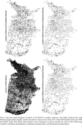
We combine the advantages of the PRISM model (good spatial interpolation) with better temporal coverage of individual weather stations (daily rather than monthly values). We do this by pairing each of the 259,287 PRISM grids that cover agricultural area with the closest seven weather stations that have a continuous record of daily observations. A station was defined to have a continuous record if at least 90% of 1950–2004 were “good” months (one with three or fewer missing daily values) and if the station was never relocated by more than 0.035° latitude or longitude. The top left panel of figure 1 shows locations of all weather stations covered by National Oceanic and Atmospheric Administration (NOAA), while the upper right panel shows locations of the 2,919 stations with continuous precipitation records for 1950–2004. The lower two panels display locations of the 1,796 stations with continuous minimum temperature records as well as the 1,818 stations with continuous maximum temperatures records.

We regress monthly averages at each PRISM cell on the derived monthly averages at each of the seven closest stations, including month-fixed effects. The R² for ordinary least squares (OLS) regressions linking minimum and maximum temperatures to the seven closest weather stations and for the Tobit regressions for nonnegative precipitation values equal 0.999 on average, which implies a very good fit.³

In a next step, we replace all missing values at our set of weather stations with interpolated values from other stations with nonmissing values. We do so by regressing daily values at each weather station on the seven closest other weather stations with nonmissing values for that day, including half-month-fixed effects.⁴ This gives a time series of daily values at each of the stationary weather stations.

The derived relationship between monthly PRISM grid averages and monthly averages at each of the seven closest stations is utilized to extrapolate the daily records at the seven closest weather stations to obtain daily records at each PRISM grid. Given estimated daily minimum and maximum temperatures, we use a sinusoidal curve to approximate the fraction of each day in each 1°C temperature interval between −5°C and 50°C. Finally, we average precipitation and time at each temperature over all PRISM grid cells in a county that have positive agricultural area. The agricultural area in each cell was obtained from a LandSat satellite image.⁵ All weather variables are summed for the six-month period March through August. Exogenously fixing this time period allows for an endogenous choice of the growing season within these months.

We pair the weather data with county-level corn yields reported by the National Agricultural Statistics Service for the years 1950–2004.

Empirical Estimates

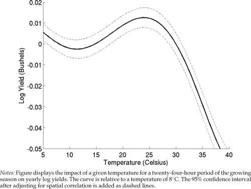
We limit the analysis to eastern counties that rely mainly on rainfall for soil moisture.⁶ We end up with 87,619 observations in 1,839 counties for 1950–2004. The fifth-order Chebychev polynomial between temperature and corn yields is displayed as a solid line in figure 2. The 95% confidence band, after adjusting for the spatial correlation of errors within years, is added as a dashed line. Impacts are normalized relative to a temperature of 8°C, that is, the y-axis displays the effect of a twenty-four-hour period at a certain temperature relative to a twenty-four-hour period at 8°C. Note how growth is increasing in temperatures between 12°C and 25°C, before it rapidly becomes negative for temperatures in excess of 30°C. One day of 38°C will lower annual corn yields by 5%. The upper bound of 30°C (86°F) when temperatures become harmful is lower than most estimates in the literature.

The quadratic functional form in precipitation exhibits an inverted U-shape with an optimal level of 26 inches, which is close to predictions from field experiments. Since we use a semilog model, the marginal value of heat depends on precipitation, as the two interact. The R² for the regression including year and county-fixed effects is 0.76.

Conclusions

An extensive literature examines the relationship between weather outcomes and corn yields. Traders of corn futures, risk-management agencies designing optimal crop insurance contracts, as well as regulators assessing the effects of climate change, require an accurate relationship between temperature and yields. In this paper, we utilize a unique fine-scale data set of daily weather records and link it to corn yields on a large geographic scale covering 1,839 eastern counties for the fifty-five years from 1950 to 2004.

We find a significant nonlinear relationship between temperature and corn yields that is roughly in line with the concept of degree days: yields are increasing in temperature for moderate temperatures, but become quickly harmful once temperatures exceed 30°C. This relationship is highly significant.

In future work, we plan to investigate whether the relationship is the same for various subregions, has remained unchanged over time and whether irrigation/high precipitation moderates the damaging effects of high temperatures.