The formation of trajectories during goal-oriented locomotion in humans. II. A maximum smoothness model
Abstract
Despite the theoretically infinite number of possible trajectories a human may take to reach a distant doorway, we observed that locomotor trajectories corresponding to this task were actually stereotyped, both at the geometric and the kinematic levels. In this paper, we propose a computational model for the formation of human locomotor trajectories. Our model is adapted from smoothness maximization models that have been studied in the context of hand trajectory generation. The trajectories predicted by our model are very similar to the experimentally recorded ones. We discuss the theoretical implications of this result in the context of movement planning and control in humans. In particular, this result supports the hypothesis that common principles, such as smoothness maximization, may govern the generation of very different types of movements (in this case, hand movements and whole-body movements).
Introduction
The existence of invariant properties of biological motion has been reported in many experimental studies, in particular those related to arm movements in animals and humans (Jordan & Wolpert, 1999). For instance, in the case of reaching and drawing experiments, stereotyped behaviours in terms of velocity profiles and smoothness of the hand trajectories in space are reported in the literature (Morasso, 1981; Atkeson & Hollerbach, 1985). This stereotypy is particularly striking in light of the theoretically infinite number of motor solutions to reach a spatial target. The existence of such motor invariants and stereotypy were proposed to be the by-product of control laws characteristic of biological systems. As a consequence, computational approaches have been developed over the past 20 years in order to formulate the principles underlying the motor control.
In the companion paper (Hicheur et al., 2007), we demonstrated for the first time that locomotor trajectories produced by humans in a simple goal-oriented task were also highly stereotyped. We also observed that this stereotypy of whole-body trajectories contrasted with a much greater variability in the feet placement. This observation indicates that goal-oriented locomotion should be considered not only at the level of the steps but also at the level of the whole trajectory. It is then necessary to develop a computational approach to provide some elements of understanding of the mechanisms underlying the generation of locomotor trajectories.
Optimal control approaches
This paper addresses this problem within the framework of optimization theory. The optimal nature of locomotor behaviour was first investigated from a biomechanical viewpoint at the level of the step formation. For instance, it has been shown that humans choose walking or running so as to minimize the metabolic energy cost at their current speed, as measured by their consumption of oxygen (Alexander, 1989).
Optimization theory is an appealing framework as it is related to the possibility that the sensorimotor system is the product of processes such as evolution, development, learning or adaptation that continuously act to improve behavioural performance (Todorov, 2004). In practice, optimality principles have been successful in modelling a great variety of biological movements.
 (1)
(1)In the above approach, the optimal trajectory is determined only by the kinematics of the hand and is thus independent of the physical system that generates the movement. Alternatively, Uno et al. (1989) proposed a minimum torque change model that takes into account dynamic properties of the arm. They modelled the arm as a two-joint manipulator controlled by torques applied at the joints, and showed that the trajectories that minimize the total squared time derivatives of the torques displayed some features of actual hand trajectories.
Recently, a number of studies have emphasized the importance of biological noise present in the motor system at many levels, ranging from the neural commands to the muscular apparatus. These studies presented computational approaches that involve a stochastic component and were successful in predicting several properties of human movements (see for instance the minimum variance model of Harris & Wolpert, 1998, or the optimal stochastic feedback control framework of Todorov & Jordan, 2002).
Minimum squared derivative (MSD) principles
 (2)
(2)Richardson & Flash (2002) conducted a comparative study in which they examined the capacities of MSD principles of different orders to predict hand trajectories. In particular, they found that 3rd- and 4th-order MSD principles (minimum jerk and minimum snap) usually performed better than those of other orders. In addition to quantitative fit, the trajectories predicted by 3rd- and 4th-order MSD principles displayed typical qualitative characteristics of human hand trajectories: smoothness of the trajectory, straight hand paths and bell-shaped velocity profiles in reaching tasks, inverse relationship between velocity and curvature in drawing tasks (the so-called two-thirds power law: Lacquaniti et al., 1983), etc.
At the trajectory level, human locomotion seems to share some of these qualitative features. Indeed, one can observe that human locomotor trajectories are generally smooth. Straight paths are also generated for reaching a spatial goal in an environment free of obstacles, provided that the initial body orientation is compatible with such a path. Finally, humans tend to decelerate in the curved parts and accelerate in the straighter parts of a trajectory. This last observation was confirmed by a recent comparative study (Hicheur et al., 2005) where the authors quantitatively examined the relationship between velocity and curvature in locomotor tasks where subjects had to walk along complex shapes. While the two-thirds exponent was not observed for these shapes (as opposed to the case of hand movements: Viviani & Flash, 1995), the inverse variations of velocity and curvature could be reproduced by multiple power laws whose exponents depended on the shape. This variability of the exponents suggested that the power laws relating the velocity to curvature in human locomotion could be by-products of more general principles, for instance the optimality principles mentioned above.
Taken together, these observations raise the possibility that MSD principles underlie the generation of human locomotion trajectories. If verified, this would suggest that the same set of principles account for different types of movements (hand movements and locomotor movements in our case) and would provide interesting theoretical insights into the understanding of the functional organization of the motor system in general. In order to test this hypothesis, we designed an experiment in which subjects had to produce a wide variety of locomotor trajectories. We then compared the experimentally recorded trajectories with the optimal trajectories predicted by four smoothness maximization models derived from the MSD approach.
Materials and methods
Experimental data
The experimental protocol is presented in detail in the companion paper. Subjects gave their informed consent prior to their inclusion in the study. Experiments conformed to the Code of Ethics of the Declaration of Helsinki. Briefly, we designed a goal-oriented locomotor task similar to a ‘walking through a distant doorway’ situation in order to observe the formation of relatively complex locomotor trajectories. We asked the subjects to walk along the laboratory-based Y-axis for about one meter before reaching the actual initial position (the origin (0,0) of the laboratory's reference frame), so that their walking direction was approximately orthogonal to the X-axis when they reached the point (0,0). They then had to walk towards and through a distant doorway (also designated below as ‘the target’) located at various positions and with various orientations (see Fig. 1). The doorway was ∼ 1 m wide, so that the subjects had no difficulty going through it at normal walking speeds. Between the point (0,0) and the target, no specific instructions were provided to the subjects relative to the path to follow. The subjects were also free to choose their walking speed over the whole trajectory.
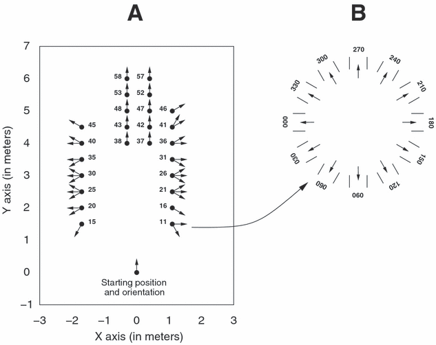
(A) Spatial disposition of the 40 tested targets. Each target position is represented by a small black disk. The possible target orientations for each target position are indicated by arrows. (B) The 12 target orientations, ranging from 0 to 330°.
In order to facilitate the analysis, we classified the 40 tested targets in four categories according to the different turning magnitudes induced by the door orientations. The four categories were: HC (high curvature), MC (medium curvature), LC (low curvature) and ST (straight; see Fig. 2 for an illustration of four typical trajectories recorded in one subject). The experimental database used for our study was composed of 709 trajectories (we had to eliminate 11 faulty trials out of the 40 targets × 6 subjects × 3 trials = 720 trials). The analysis was performed on the time interval separating the instant t0 when subjects crossed the X-axis and the instant t1 when they reached the centre of the door, according to the task requirements (see Fig. 2). The trajectory was then time-rescaled so that t0 = 0 and t1 = 1.
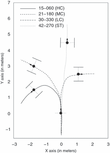
Four actually recorded trajectories, one trajectory per category.
Modelling approach
As mentioned in the introduction, MSD principles have proved to be particularly relevant for modelling hand movements. In order to test how such smoothness-based principles can predict locomotor trajectories, we constructed mathematically MSD trajectories as follows.
 (3)
(3) (N corresponds to the number of trajectories recorded for this target).
Some of these 12 parameters were task-related and thus were not related to any spontaneous strategy. Indeed, according to the experimental protocol, the initial and final positions (x0, y0, x1, y1) corresponded, respectively, to the origin of the laboratory's reference frame and to the centre of the door. Similarly, the initial movement direction was imposed as parallel to the Y-axis while the final movement direction was constrained by the orientation of the door. As subjects were carefully monitored during the session, the extracted values of these parameters were very close to the imposed ones: over the 709 trajectories, the average distance (± SD) between the actual and the imposed initial positions was 3.0 ± 2.5 cm, the average distance between the actual and the imposed final positions was 3.2 ± 2.2 cm, the average absolute difference between the actual and the imposed initial orientations was 9.6 ± 7.9° and the average absolute difference between the actual and the imposed final orientations was 5.9 ± 4.4°. Thus, our choice to extract these values from the data rather than to compute them a priori from the task was only motivated by convenience.
In contrast, initial and final accelerations ( ) and initial and final speeds (the norms of the velocity vectors) were not imposed by the task and thus contained information about the subjects' movement strategies or their personal preferences. Considering these parameters as free parameters in the optimization procedure yielded close-to-zero values, which was not consistent with the observations. On the other hand, estimating them by an independent method would be complicated and not relevant with respect to our objectives (see Discussion for more details on the issue of putting experimental values into the models).
At a computational level, as our objective consisted of predicting the whole trajectory kinematics (path and velocity profile), these values actually contained relatively little information. In contrast, the original two-thirds power law (Lacquaniti et al., 1983), the modified two-thirds power law (Viviani & Schneider, 1991) or the constrained minimum jerk model (Todorov & Jordan, 1998) aimed at predicting only the velocity profile. Moreover, these models required as inputs the entire recorded path in conjunction with either the end-point velocities and accelerations (for the constrained minimum jerk model) or the entire velocity profile (for the modified two-thirds power law). However, it should be recognized that some of the trajectories studied in the references cited above were rather more complex than ours.
It should also be noted that the movement duration was implicitly extracted in the time-rescaling procedure.
 (4)
(4)Performance of the models
We performed a series of quantitative comparisons between the actual and the predicted trajectories either at the global level of the trajectory or at the more detailed level of the velocity profile.
In the companion paper, similar comparisons were conducted in order to assess the stereotyped behaviour of actual trajectories corresponding to a single task. For this, the average trajectory was compared to actual trajectories, resulting in several measurements [e.g. average and maximal trajectory deviations (ATD and MTD) and average and maximal velocity deviations (AVD and MVD)].
Here, we were interested in the predictive capacities of our models. We thus compared the average trajectory corresponding to a given task to the trajectories predicted by our models for the same task. This was reasonable as actual trajectories were stereotyped and, consequently, very similar to the average trajectory.
Trajectory prediction
 (5)
(5) (6)
(6) (7)
(7)For each category X (X = HC, MC, LC, ST), the average ATEc and MTEc over all targets belonging to this category were denoted, respectively,  and
and 
For a graphical examination of the models' performances, we also plotted in 3-6 the variance ellipses calculated by principal component analysis. Intuitively, the variance ellipse at time t is centred at (xav(t),yav(t)) and its orientation and magnitude indicate how the (xi(t),yi(t)) (i = 1…N, where N corresponds to the number of trajectories recorded for this target) are distributed around (xav(t),yav(t)). Note that r1(t)2 + r2(t)2 = TD(t)2 where r1 and r2 are the lengths of the ellipse's semi major and semi minor axes and TD is the trajectory deviation defined in the companion paper.
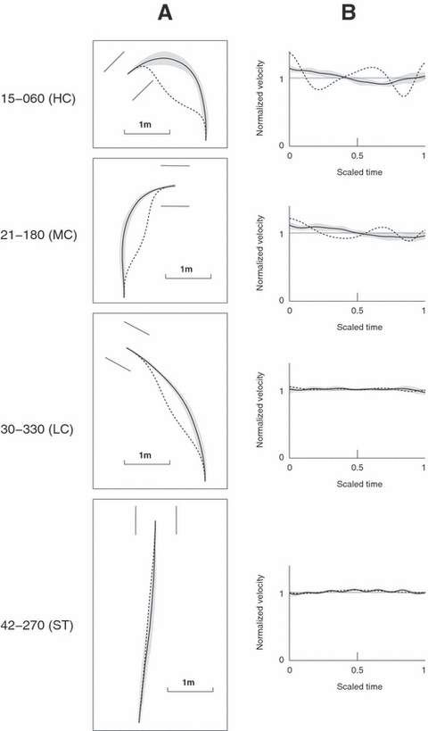
Prediction of the minimum velocity model for four representative trajectories. (A) Geometric paths of the average (solid lines) and the predicted (dashed lines) trajectories. The variance ellipses (in grey) are also plotted in order to show the spatial variability around the average trajectory at every time instant (see Materials and methods). (B) Normalized velocity profiles of the average (solid lines) and of the predicted (dashed lines) trajectory. The standard deviation around the average velocity profile is shaded in grey. The dark grey horizontal line shows the mean value (in time) of the normalized velocity profiles.

Prediction of the minimum acceleration model for four representative trajectories. For details, see legend of Fig. 3.
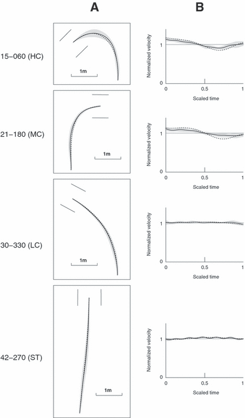
Prediction of the minimum jerk model for four representative trajectories. For details, see legend of Fig. 3.
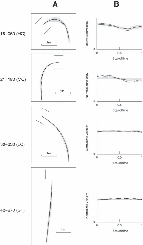
Prediction of the minimum snap model for four representative trajectories. For details, see legend of Fig. 3.
Velocity profile prediction
In contrast to the companion paper, the goal here is to compare the velocity profiles in terms of their variations in time rather than in terms of their absolute variabilities (which are due in part to the variability of the walking tempos in different subjects; these have been measured in the companion paper).
 (8)
(8) (9)
(9) (10)
(10) (11)
(11) (12)
(12) (13)
(13) (14)
(14) (15)
(15) and
and 
Statistical analysis
We performed repeated-measurements anova with the Statistica 5.1 software package (Statsoft ®) in order to compare statistically the performance of the models. More specifically, given two models, we compared their maximum trajectory errors in order to assess whether one model was significantly better than the other. We also tested whether the maximum trajectory errors of a model were significantly smaller or greater than the corresponding maximum trajectory deviations (the experimental variabilities).
Results
Qualitative examination
Minimum velocity model
In Fig. 3, we plotted the predictions of the minimum velocity model for four representative targets, one for each category. We observed that the geometric paths predicted by this model tended to be the straightest possible. Thus, the predicted paths for the targets of category ST were accurate. However, for the targets that required some amount of curvature (HC, MC and LC), the predicted paths were strongly bent towards the interior of the curve, resulting in a big inaccuracy around the middle of the path.
Minimum acceleration model
Predictions of the minimum acceleration model are presented in Fig. 4. Qualitatively, for categories HC, MC and LC, the geometric paths predicted by this model were much more accurate than those predicted by the minimum velocity model. However, the predictions were still not satisfactory for categories HC and MC, which included the most curved trajectories. Indeed, as in the minimum velocity model, the predicted paths for these categories tended to be straighter than the actual paths. More specifically, in the regions of relatively high curvatures, the predicted paths fell outside the grey area of the variance ellipses, implying that their distances to the average paths were greater than the experimental variability in these regions.
The comparison of the velocity profiles only makes sense when the geometric paths are similar, i.e. in the case of category ST for the minimum velocity model and in the case of categories LC and ST for the minimum acceleration model. In these cases, the average velocity profiles were almost constant in time, which was well reproduced by both models.
Minimum jerk and minimum snap models
The predictions of these models are presented in 5, 6, respectively. We first observed that the trajectories predicted by the two models were very similar for the four representative targets. In contrast to the two previous models, the geometric paths predicted by these two models for the HC and MC trajectories are smoothly curved and bear impressive resemblance with the average ones. As an illustration, the predicted paths always lay inside the grey area of the variance ellipses, implying that the distance between the predicted and the average paths was smaller than the experimental variability at every time instant.
At the level of the velocity profiles, we noted that the average velocity profiles were approximately constant in time for categories LC and ST (the only minor variations were due to the step-level oscillations). This was well reproduced by both models. For categories HC and MC, in the average velocity profile, the velocity decreased and became minimal around t = 0.7 (where t is time scaled from 0 to 1) before increasing again. This variation of the velocity was related to the variation of curvature in the corresponding geometric paths. The inverse relationship in human locomotion has been experimentally observed by Vieilledent et al. (2001) and by Hicheur et al. (2005). The predicted velocity profiles successfully captured this behaviour, although with some slight overshoot. For instance, for category HC the velocity profile of the minimum jerk trajectory had almost the same global behaviour as the average one: both decreased and became minimal around t = 0.7 before increasing again. However the variations in the predicted profile were slightly larger than the variations in the average profile.
Quantitative examination
We next proceed to a more precise, quantitative comparison between average and predicted trajectories.
Trajectory errors
The average and maximal trajectory errors as defined in Methods are plotted in Fig. 7. As noted above, the minimum velocity model (dark grey bars) produced acceptable predictions only in the case of straight trajectories (category ST). As soon as the targets imposed some amount of trajectory curvature (categories LC, MC and HC), the minimum velocity trajectories differed completely from the actual trajectories.
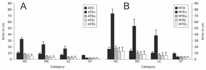
(A) Average and (B) maximal trajectory errors (ATE and MTE; the suffixes v, a, s, j refer, respectively, to velocity, acceleration, jerk and snap) in centimetres: dark grey bars for minimum velocity, medium grey bars for minimum acceleration, light grey bars for minimum jerk and white bars for minimum snap, averaged over targets corresponding to the same category. For comparison, the average and maximal trajectory deviations (ATD and MTD) are also plotted (black bars).
The minimum acceleration principle (medium grey bars) performed somewhat better but for categories HC and MC it was still not satisfactory. For example, the average maximal prediction error over the 20 targets belonging to these categories,  (14.7 cm), was not significantly different (F1,19 = 0.27, P > 0.01) from the corresponding experimental variability (black bars) MTDHC+MC (15.1 cm).
In contrast, minimum jerk (light grey bars) and minimum snap (white bars) principles provided strikingly good predictions. In fact, as noted above, the predictions of minimum jerk and minimum snap models were mostly similar. As a matter of fact, the largest difference between the two models was observed for target 31–150 (category HC), where the maximal distance between the two predicted trajectories was 3.6 cm. Over the 20 targets of categories HC and MC, the average (± SD) maximal distance between minimum jerk and minimum snap trajectories was only 2.1 cm (± 0.6 cm).
Even in the case of the highly curved trajectories of category HC, the distance between the average trajectory and the minimum jerk trajectory was < 13 cm over the whole trajectory ( = 12.7 cm). As the average trajectory length for this category was 3.7 m, this corresponds to a maximal error of only 3.4%. Moreover, the prediction errors of the minimum jerk and minimum snap models were smaller than the experimental variability. For categories HC and MC,
  (10.3 cm) was significantly smaller (F1,19 = 20.7, P < 0.01) than MTDHC+MC (15.1 cm). This result is related to our previous qualitative observation that the paths predicted by these models always lay inside the variance ellipses.
Next, the respective performances of minimum acceleration, minimum jerk and minimum snap models were compared over the 20 targets belonging to categories HC and MC (we observed that the three models yielded similar performance for the straight and close-to-straight trajectories ST and LC). The average maximal prediction error over these targets were  , 14.7 cm;
  , 10.3 cm; and
  , 10.7 cm. The difference between the minimum acceleration and minimum jerk average MTEs was statistically significant (F1,19 = 29.10, P < 0.01). The difference between the minimum jerk and minimum snap average MTEs was also significant, albeit to a lesser extent (F1,19 = 9.80, P < 0.01).
The superiority of minimum jerk and minimum snap models over minimum acceleration and minimum velocity models can be explained as follows. Minimizing the mean squared velocity cost is almost equivalent to finding the shortest path, i.e. the straightest path in Euclidean geometry, that satisfies the boundary conditions. This prevents the minimum velocity model from predicting accurate trajectories as soon as the targets required some amount of curvature. As for the minimum acceleration model, the mean squared acceleration cost penalises, by definition, large variations in time of the velocity vector. This is not consistent with the experimental observation of significant variations in the velocity vector (in particular, the variations in the orientation of this vector) around the regions of high curvature in MC and HC trajectories. In contrast, minimum jerk and minimum snap allow more flexibility for the variations in the velocity vector and are thus more capable of generating smoothly curved trajectories.
Velocity profile errors
The average and maximal normalized velocity errors as defined in Materials and Methods are plotted in Fig. 8. These errors in terms of the velocity profile followed the same tendency as those in terms of trajectory kinematics: in all categories, the velocity profiles of minimum jerk (light grey bars) and minimum snap (white bars) trajectories deviated very slightly from the average velocity profiles. Even for category HC, the average normalized velocity error was only 6% (of the average actual velocity) while the maximal normalized velocity error over the trajectory was < 12%. In absolute terms, these errors were close to the same order of magnitude as the experimental variability (black bars).
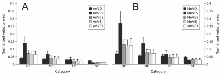
(A) Average and (B) maximal normalized velocity errors (AnVE and MnVE; the suffixes v, a, s, j refer, respectively, to velocity, acceleration, jerk and snap): dark grey bars for minimum velocity, medium-grey bars for minimum acceleration, light-grey bars for minimum jerk and white bars for minimum snap, averaged over targets corresponding to the same category. For comparison, the average and maximal normalized velocity deviations (AnTD and MnTD) are also plotted (black bars). In the process of computing the above quantities, all velocity profiles were normalized so that their average values over the movement duration equals 1 (see Materials and methods).
Discussion
Despite the great number of possible trajectories to reach a distant doorway, humans exhibit stereotyped behaviour in terms of both path geometry and trajectory kinematics (see companion paper). This suggests that some underlying principles may govern the formation of whole-body trajectories in space. In the present study, we developed a comparative approach in which we tested four optimization models already studied in the literature in the context of hand trajectory generation (Richardson & Flash, 2002). To assess their validity, we applied these models to a wide range of locomotor tasks involving trajectories of various lengths and curvatures. Through qualitative and quantitative examinations, we established that two out of the four models, namely the minimum jerk and the minimum snap models, provided predictions remarkably close to actual trajectories, at both the geometric and the kinematic levels.
Predictive power of the models
As pointed out by Todorov & Jordan (2002), the predictive power of a model is not only measured by how well it fits the experimental data. At least two other characteristics must be taken into account. The first characteristic is the quantity of information that needs to be extracted from the experimental data. Obviously, the less information extracted from the data, the greater the challenge for the model. In order to predict the velocity profiles of curved hand movements, the constrained minimum jerk model requires, as inputs, the entire movement path and the initial and final velocities (Todorov & Jordan, 2002). Viviani & Flash (1995) used experimental values of the velocity and acceleration at several via-points in order to predict the velocity profiles in curves drawing tasks. In contrast, our models (which predict both the path and the velocity profile) were required to extract only a small number of parameters, namely the initial and final speeds and accelerations, and the movement duration (see Materials and methods). The last parameter was extracted in the time-rescaling procedure, which normalizes the durations of actual and simulated trajectories. This procedure is pervasive in the literature (Flash & Hogan, 1985; Uno et al., 1989; Harris & Wolpert, 1998; Todorov & Jordan, 1998; Richardson & Flash, 2002) but, in light of our current discussion, it also reduces the predictive power of the model. Recently, Tanaka et al. (2006) proposed a variation of the minimum variance model (Harris & Wolpert, 1998) that was able to determine the movement duration from a first principles approach. The authors considered the movement duration as a parameter to be optimized, and performed the subsequent optimization under the constraint that the movement achieves a predetermined level of accuracy. Within our experimental protocol, the determination of the movement duration and, more generally, the issue of speed–accuracy tradeoff in human locomotion could not be satisfactorily investigated; testing different walking speeds and varying the constraints on the spatial accuracy (e.g. varying the size of the doorway) will help in addressing these questions in future studies.
 (16)
(16)Accuracy demands and smoothness of the trajectories
Also related to the above discussion on the speed–accuracy tradeoff is the relationship between the task's accuracy demands and the smoothness of the resulting trajectories. Sosnik et al. (2006) have reported that stringent accuracy demands resulted not only in an increased movement duration but also in a decreased movement smoothness. In our experiments, the doorway was large enough (see Materials and methods) that it allowed subjects to get through without any difficulties at normal walking speeds, resulting in smooth trajectories, as we observed. Again, varying e.g. the size of the doorway in future experiments will help in further exploring the relationship between the accuracy demands and the smoothness of the resulting locomotor trajectories.
The role of online control in the implementation of locomotor trajectories
Although trajectories corresponding to a given task were highly stereotyped, there still existed a small trial-to-trial variability, ranging between 10 and 15 cm for the straight and highly curved trajectories, respectively (see the companion paper). This variability could be related to morphological differences between the subjects and to the noise present in the human sensory and motor systems (Harris & Wolpert, 1998).
Remarkably, the variability was smaller at the beginning and the end of the trajectory and larger in between (see for instance the HC trajectory in Fig. 3A). If the movement was executed in open-loop (i.e. in a purely feedforward manner), the variability would increase throughout the movement. Thus, the observed variability pattern indicates that an online feedback control process is at work during the implementation of the optimal trajectory (presumably according to a minimum jerk or minimum snap criterion, as suggested by our results). The nature of such a control process is, however, less clear. In the case of hand movements, a number of hypotheses have been proposed, including trajectory-tracking mechanisms through servo control (McIntyre & Bizzi, 1993) or optimal feedback control schemes (Todorov & Jordan, 2002). Within this context, increasing the complexity of the goal-oriented task (for instance using a multiple via-points task, as in Todorov & Jordan, 2002), applying external perturbations during the movement execution or testing specifically the contribution of sensory information (for instance by manipulating the visual inputs with prism glasses, as in Rushton et al., 1998) will help in unveiling the nature of the online control process at work during the implementation of locomotor trajectories.
Common strategies may govern the formation of hand and whole-body trajectories
As evoked in the companion paper, recent studies suggest that the generation of hand and whole-body movements share common strategies. For instance, Papaxanthis et al. (2003) have recently observed that vertical whole-body and arm movements executed in the sagittal plane share kinematic similarities. The authors then suggested that the central nervous system (CNS) uses similar motor plans for the performance of arm and whole-body movements in the sagittal plane. The comparison of the velocity–curvature relations in human locomotion and in hand movements has also been conducted, using the same (up to a scaling factor) predefined curved paths in both types of movements (Hicheur et al., 2005). At the computational level, Harris & Wolpert (1998) tested the assumption that the CNS learns a new movement by minimizing the variance of the final effector position for both hand and eye movements.
In this context, our observation that the minimum jerk and minimum snap models best predict locomotor trajectories should be related to the case of hand movements, where very similar results have been reported (Flash & Hogan, 1985; Richardson & Flash, 2002). For instance, in the task of periodic drawing of closed shapes, Richardson & Flash (2002) showed that MSD models of order n > 2 provided more accurate predictions than MSD models of lower orders.
However, hand and whole-body movements differ greatly in their spatial and temporal scales: for instance, hand trajectories are usually tens of centimetres long while travelled distances during locomotor tasks are usually > 10× longer. This difference in magnitude is associated with a difference in the nature and the number of muscles involved in the production of the movement: while hand movements activate mostly the arm muscles, locomotor activity mobilizes most of the body muscles (lower limbs muscles for body propulsion, upper body muscles for trunk stabilization, neck muscles for steering, etc.). Thus, the fact that the same models could account for both hand and whole-body movements is a striking observation and strongly supports the hypothesis that common mechanisms (in our case, maximizing movement smoothness) are implemented by the motor system in the generation of various types of movements. More specifically, this hypothesis could be related to a theory put forward by Bernstein (1967), according to which there exist, at the higher levels of the motor system, kinematic representations of movements that are independent of the nature (in our case, the arm or the whole locomotor system) of the actual effector.
The nature of the control variable(s)
The last remark is associated with the conceptual distinction between kinematic and dynamic variables usually presented in the literature (Jordan & Wolpert, 1999). While kinematic variables (e.g. the hand's position, velocity, acceleration, jerk, etc. measured in the laboratory reference frame) describe the movement of the end-effector in the extracorporeal space, dynamic variables (e.g. the torques applied at the joints, the muscle activations, etc.) are related to the internal mechanical properties of the motor system.
In the case of arm movements, the motor apparatus can be realistically modelled by a two-link manipulator controlled by torques applied at the joints (Uno et al., 1989). In this context, the opposition between kinematic control of the end-effector (the hand) and dynamic control of the torques can be readily investigated. For locomotion, however, given the greater dimensionality of the motor system (at the segmental, muscular, etc. levels), there is a theoretically greater complexity of the motor control problem. Thus, the issue of identifying precisely which variables are being controlled could not be satisfactorily addressed in this study; testing other locomotor tasks and using different kinds of perturbations will help in further exploring the mechanisms underlying the generation of locomotor trajectories. Nevertheless, two series of observations argue in favour of a kinematic control of goal-oriented locomotion. First, we provided evidence in the companion paper that locomotor trajectories are stereotyped, in particular at the kinematic level. In the present study, we were able to accurately predict locomotor trajectories with kinematic-based models. While this does not rule out the possibility that the CNS may take into account dynamic variables in the generation of locomotor trajectories, we suggest that dynamic variables are rather used at the motor implementation level. Following this idea, the transformation from kinematic objectives into dynamic strategies may be acquired with learning (see also Winter & Eng, 1995).
Finally, it should be noted that, contrary to the case of hand movements where the laboratory (allocentric) reference frame (RF) and the body (egocentric) RF are equivalent, here the body RF moves and turns with respect to the laboratory RF when the subject is moving. In this context, the kinematic quantities used in our models (the position of the subject and its derivatives) are only interesting when computed in the laboratory RF as, in his body RF, the subject's position is constant in time. From a theoretical viewpoint, while egocentric and allocentric strategies for spatial navigation and spatial memory are usually debated in the literature (see Berthoz & Viaud-Delmon, 1999), the question of which RF(s) are actually used for the planning and control of goal-oriented locomotion has received little attention. Here, our results suggest that whole-body trajectories are optimized in the laboratory RF. However, further refinements of our experiments and models will also have to consider the possibility of egocentric components in the mechanisms underlying the formation of whole-body trajectories.
An integrative approach for the study of human locomotion
While our approach focused on the global, trajectory-level, descriptions, some fine-grained properties of the locomotor activity can be captured only if the step-level parameters are taken into account. For instance, the variations of the tangential velocity during the step cycle must be included in our models in order to account for the small oscillations observed in the velocity profiles (see for example the average velocity profile corresponding to target 42–270 in Fig. 3B).
Recently, Arechavaleta et al. (2006) proposed a robotics-inspired approach that emphasized the nonholonomic nature of human locomotion. For a wheeled vehicle (e.g. a bicycle, a car, a car with trailers, etc.), the kinematic constraint that forces the vehicle to move in the direction of its main axis is known as being nonholonomic (Laumond, 1998). This constraint dramatically reduces the possible movements of the vehicle and, as a result, it strongly affects the nature of the vehicle's optimal trajectories. For instance, as a wheeled vehicle cannot move sideways, the quickest way to parallel park is not associated with a straight path (as it would be in the usual geometry) but consists rather of a series of complicated manoeuvres. In the context of human locomotion, this constraint was interpreted as forcing the subject to move in the direction of his ‘axis’, which was defined as the orthogonal direction to the shoulders' segment. This constraint was partly verified experimentally (see Arechavaleta et al., 2006 for more details). However, in the models presented here, we did not take into account the body orientation and the related nonholonomic constraint. Nevertheless, our models could predict the trajectories with great accuracy, which suggests that, for the range of turning amplitudes tested in our experiments, the body orientation may not be a determining factor in the generation of locomotor trajectories. For more demanding tasks (involving for instance very narrow turns), it is likely that constraints on the body orientation such as the nonholonomic one exert a positive effect on the whole-body trajectories. Both experimental and theoretical issues regarding the integration of such elements into our models are the subject of ongoing research.
Acknowledgements
This study was supported by Human Frontiers grant n° R6P0054/2004. We thank Professor D. Bennequin and Dr S. I. Wiener for helpful comments. We are also grateful to two anonymous reviewers whose suggestions have greatly improved the manuscript.
Abbreviations
-
- AnVD
-
- average normalized velocity deviation
-
- AnVEc
-
- average maximal normalized velocity error
-
- ATD
-
- average trajectory deviation
-
- ATEc
-
- average trajectory error
-
- AVD
-
- average velocity deviation
-
- HC
-
- high curvature
-
- LC
-
- low curvature
-
- MC
-
- medium curvature
-
- MnVD
-
- maximal normalized velocity deviation
-
- MnVEc
-
- maximal normalized velocity error
-
- MSD
-
- minimum squared derivative
-
- MTD
-
- maximal trajectory deviation
-
- MTEc
-
- maximal trajectory error
-
- MVD
-
- maximal velocity deviation
-
- nVD
-
- normalized velocity deviation
-
- ST
-
- straight
-
- TEc
-
- instantaneous trajectory error. Subscripts
-
- a
-
- minimum acceleration
-
- av
-
- average
-
- c
-
- (subscript) standing for v, a, j or s
-
- j
-
- minimum jerk
-
- s
-
- minimum snap
-
- v
-
- minimum velocity.
Appendix
 (17)
(17) (18)
(18)Minimum jerk trajectories
 (19)
(19)Minimum snap trajectories
 (20)
(20)Minimum velocity and minimum acceleration trajectories in restricted solutions space
If n ≤ 2, the problem is ill-posed (Harris & Harwood, 2005) in the sense that no optimal trajectory exists. However, if we restrict the solution space to the set of polynomials of degree less than or equal to d (where d is an integer ≥ 6), then we can find a unique optimal trajectory xd. As d grows, the cost associated with xd decreases (because the solution space is larger). However, when d→∞, xd converges to a trajectory that no longer verifies the boundary conditions.
As minimum jerk and minimum snap principles yield polynomials of degrees less than or equal to 7, we set d = 7 in order to make unbiased comparisons of the four models.
 (21)
(21) (22)
(22)The case n = 1 (minimum velocity) can be treated similarly.


