Modelling the relationship between sexual reproduction and rhizome growth in Posidonia oceanica (L.) Delile
Abstract
The relationship between flowering and growth performance of Posidonia oceanica (L.) Delile in meadows distributed along the south-eastern coast of Sicily (Italy) was investigated by means of a statistical model (generalized linear mixed model) combined with the lepidochronological analysis. Over a 28-year period, 67 floral stalk remains were observed. The highest flowering index was recorded in lepidochronological year 1998 (10.1%) and the Inflorescence Frequency per age showed a clear decrease corresponding to 15-year-old shoots. The sexual reproductive event had positive effects on rhizome elongation (cm year−1) and leaf production (no. leaves year−1) in the same flowering year, whilst no effect on the rhizome production (mg year−1) was observed. Rhizome growth variables showed significant negative lagged responses in the two years following flowering. On the whole, we calculated that the effect exerted by flowering, in terms of loss on rhizome elongation and production, was about 27% and 38%, respectively. Although it has been demonstrated that recovery from the stress induced by sexual reproduction is limited to the two years after flowering, the magnitude of the reproductive cost may become quite considerable especially in comparison with the whole lifespan of individual shoots.
Problem
Clonal plants can reproduce both asexually and sexually. However, they are often characterized by reduced sexual reproduction when compared with non-clonal species (Eriksson 1997). In seagrasses, which are clonal marine plants, sexual reproduction is due to both the need for dispersal and colonization of new coastal habitats (e.g. in Posidonia oceanica, Cymodocea nodosa, Zostera noltii) and to gain the benefits from genetic variation (Buia & Mazzella 1991; Gavino et al. 2000; Waycott et al. 2006), while dominant vegetative reproduction is important for meadow maintenance of most seagrass beds (Hemminga & Duarte 2000). Currently, sexual reproductive events have been observed in many species more frequently than before and often simultaneously across large spatial scales (Inglis & Lincoln Smith 1998), owing to both increased field observations (Duarte 1999) and the use of reconstructive methods allowing researches to detect and date the past flowering episodes (Pergent 1990; Duarte et al. 1994).
Posidonia oceanica (Linnaeus) Delile, a seagrass endemic to the Mediterranean Sea, forms extensive meadows that are considered as biological indicators of water quality and thus used in monitoring marine environment programmes (Casazza et al. 2002; Pergent-Martini et al. 2005). Posidonia oceanica is characterized by a low genetic variability (Procaccini et al. 2001), which is mainly due to the predominance of clonal reproduction. Nevertheless, its flowering occurs throughout the whole western Mediterranean basin (Diaz-Almela et al. 2006). More specifically, flowering is more frequent and even annual in the southern and eastern regions of the basin (Buia & Mazzella 1991) than it is along its north-western shores (Pergent & Pergent-Martini 1990; Boyer et al. 1996; Bussotti & Guidetti 1996; Stoppelli & Peirano 1996; Balestri & Cinelli 2003). The flowering of P. oceanica has a patchy distribution (Pergent 1985; Buia & Mazzella 1991) and appears generally on orthotropic rhizomes but, under particularly favourable flowering conditions (e.g. blooms of 2003), plagiotropic rhizomes could also bear flowers (Balestri et al. 2005).
In the literature, much attention has been focussed on the exogenous (such as light, temperature, hydrodynamic regime) and endogenous factors (such as shoot age, size, genetic variation, distribution of active meristems) influencing reproductive events (Thelin & Boudouresque 1985; Pergent & Pergent-Martini 1990; Buia & Mazzella 1991; Bussotti & Guidetti 1996; Balestri & Vallerini 2003; Buia et al. 2005).
Some authors observed that flowering induces some changes in the biometrical characteristics of the epigeal compartment: i.e. a reduction in leaf width, an increase in the length of older leaves and a reduction in the length and number of intermediate and young leaves (Panayotidis 1986; Pergent & Pergent-Martini 1988; Tomasello et al. 1994; Gobert et al. 2001). As to the hypogeal compartment, few remarks have been made on changes in the growth variables of P. oceanica during the same flowering year (Pergent 1987) as well as 1 year before and 1 year after the sexual reproductive event (Balestri & Vallerini 2003; Buia et al. 2005). Although the latter studies adopted a consistent methodological approach and temporal scale, results pertaining to the effects of flowering on growth performances seem to differ. Moreover, the hypothesis about some possible effects occurring for a timescale longer than 1 year remains still totally unexplored.
In this study, we evaluated the presence and duration of the effects of flowering on current and future vegetative growth in terms of rhizome production and elongation and leaf production. Hence, to achieve this purpose, a generalized linear mixed model (GLMM) was applied to time data collected at plant level in four different meadows along the coasts of Sicily (Italy). Moreover, in order to draw valid inferences about the most interesting effects, we have been also required to consider the possible effects of other variables that could play the role of confounders (Tomasello et al.in press) in the analysis.
Material and Methods
The present study was carried out between 2001 and 2002 along the south-eastern coasts of Sicily, between Cape Passero and Cape Murro di Porco (Fig. 1). In this area, benthic habitats are mainly represented by meadows of P. oceanica. The seagrass bed shows a continuous distribution covering about 8775 ha (51% of the interested area) and reaching a maximum depth of 35 m (AA. VV. 2002).
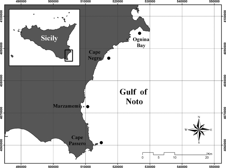
Study area, with location of the studied Posidonia oceanica meadows.
More specifically, four sites were sampled in the survey: Ognina Bay, Cape Negro, Marzamemi and Cape Passero (Fig. 1). In each site, from 80 to 120 orthotropic (vertical) shoots, attached to plagiotropic (horizontal) rhizome portions, were randomly collected by SCUBA diving at depth between 10 and 15 m. Shoots were sampled at a distance of at least 1 m to reduce the likelihood of gathering shoots connected to the same plagiotropic axis, as described by Pergent et al. (1983).
Samples were studied using lepidochronological analysis (Pergent 1990). This technique, based on the observation of the cyclic variations in the sheath thickness along the rhizomes of P. oceanica, allowed us to isolate and date rhizome segments corresponding to a 1-year period (lepidochronological year). Each lepidochronological year was determined starting to date from the rhizome apex downward and then matching the cycle of sheath thickness with the corresponding rhizome segment. This method made also possible to detect the previous shoot flowering episodes by finding floral stalk remains between the sheaths (Pergent et al. 1989). Moreover, it was possible to determine the lepidochronological year corresponding to the cycle along the rhizome where the floral stalk remains were found (Pergent et al. 1989). Conventionally, the lepidochronological year corresponds to the period when leaves have completed their growth cycle, rather than to that when they are still growing (Pergent 1990). Hence, a flowering dated, for example, in lepidochronological year 1995 indicates that the reproductive period occurred between autumn 1994 and spring 1995.
Dry weight (by weighting after 24 h at 105 °C; Duarte et al. 1997), length and number of sheaths were measured for each annual rhizome segment. Finally, the age of each rhizome segment was determined by counting the number of years between the bearing axis and the rhizome segment under study (Pergent & Pergent-Martini 1990). Hence, rhizome elongation (mm year−1), rhizome production (g dw year−1), leaf production (no. leaves year−1) and shoot age (year) were estimated.


We set out exploring the relationship between vegetative growth (rhizome production and elongation and leaf production) and flowering, lepidochronological year and age by a simple graphical representation (boxplots). Moreover, as for flowering, the three response variables were compared between shoots with and without flowering in lagged form, i.e. whether growth in a given year t is influenced by flowering in the same year t, and/or by flowering 1 year before (t − 1) and 2 years before (t − 2). As an example, let us consider the lepidochronological year 1998: in this paper, we examine whether flowering in year 1996 (t − 2), 1997 (t − 1) and 1998 (t) have had an effect on vegetative growth in the year 1998 (t). Clearly, the analysis of both simultaneous (growth and flowering at the same year t) and lagged effects (growth at year t, flowering at year t − 1 and t − 2) are carried out for each year t, so covering the whole period of interest.
Subsequently, a GLMM (Crawley 1993; Fahrmeir & Tutz 1994) was applied in order to assess the possible effects of flowering on rhizome production and elongation and leaf production. According to the exploratory analysis, this statistical model considered both the simultaneous and the lagged effects. Shoot age, lepidochronological year and site were included in the model as covariates in order to draw correct inferences about the most significant effects. Lepidochronological year and site were considered as proxy including all environmental explanatory variables varying respectively in time and space.
The GLMM dealt with the following features of the data:
- •
the non-Normality distribution of the three responses: elongation and production of rhizome are continuous variables with a strong positive asymmetry (Marbà & Duarte 1997) and leaf production is a discrete counting variable; therefore, the assumption of Normality is inappropriate for all of them;
- •
the different mathematical nature of the explanatory variables: age and lepidochronological year are continuous and presumably produce non-linear effects on the responses (Duarte 1991; Hemminga & Duarte 2000), whilst site and flowering are categorical;
- •
time dependence in the data: lepidochronological measures on the same shoot represent an instance of longitudinal dataset, with an autocorrelation structure in time which cannot be ignored for a sound statistical analysis.
The model was based on the following assumptions:
- •
the rhizome elongation and production have a Gamma distribution and leaf production has a Poisson distribution;
- •
the link function is logarithmic;
- •
the intercepts for each shoot are assumed to be random effect, in order to detect the shoots natural heterogeneity (which is unexplained by the explanatory variables) and to consider the temporal autocorrelation of the lepidochronological measurements on the same shoot.

 ); consequently, the variance
  can be interpreted as a measure of heterogeneity among shoots; Fit, Fi(t-1), Fi(t-2) are binary variables: Fit = 1 if shoot i flowered at time t, Fit = 0 if shoot i did not flower at time t; similarly for the lagged variables Fi(t-1), Fi(t-2); Ait is the age of shoot i at time t; Lt = 1986 + t is the lepidochronological year at time t.
As far as the time indexes (t, t − 1, t − 2) are concerned, the notation in the model is ‘centred’ on the response variable: we fix attention on the growth performance at time t and try to model whether it has been influenced by flowering at the same time t, flowering 1 year before (t − 1) and flowering 2 years before (t − 2). This is consistent with the standard notation used in time series analysis (see, for example, Scheiner & Gurevitch 2001).
For all three response variables (rhizome elongation, rhizome production and leaf production) only the results concerning the ‘best’ GLMM fitted to the data have been reported. This model has been selected by means of a model selection procedure based on the Akaike Information Criterion (Akaike 1973). Moreover, within the ‘best’ model, the significance of each effect on each variable has been assessed by using approximate Wald test, computed as the ratio between the estimate and its standard deviation. The values of such test statistics are indicated as ‘t-ratios’; the approximate p-values attached to them are provided by the R function glmm. In order to obtain identifiable parameters in the parameterization here used for the GLMM, it was required to refer all results to the intercept, a baseline conventional category that, in our case, was coincident with the Marzamemi site. Finally, the statistical model outcomes were also expressed on the original scale in order to simplify data interpretation.
All statistical analyses have been carried out using R vers. 2.0, a free software environment for statistical computing and graphics (downloadable at the URL http://www.r-project.org/).
Results
The lepidochronological analysis allowed us to isolate and to date 3920 rhizome segments in the 420 shoots examined. This study dealt with samples belonging to a temporal range from 1974 to 2002, excluding the years 2001 and 2002 from the data analysis as the lepidochronological growth cycle was not complete in all the shoots sampled (Peirano 2002).
As a whole, 67 floral stalks remains were detected as follows: 19 at Ognina Bay, 21 at Cape Negro, 14 at Marzamemi and 13 at Cape Passero, respectively. Flowering episodes were found only in 5 of 28 years analysed, with a higher FI in 1987, 1995, 1998, when the maximum value of 10.1% was recorded in the latter. However, it has been shown that flowering appeared to occur annually over the past few years (Fig. 2). The IF increased with shoot age up to 15 years, when the maximum IF (12.7 %) was recorded, and then declined (Fig. 3).
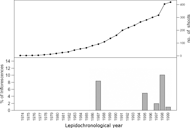
Number of shoots analysed and the flowering index in relation to lepidochronological year.
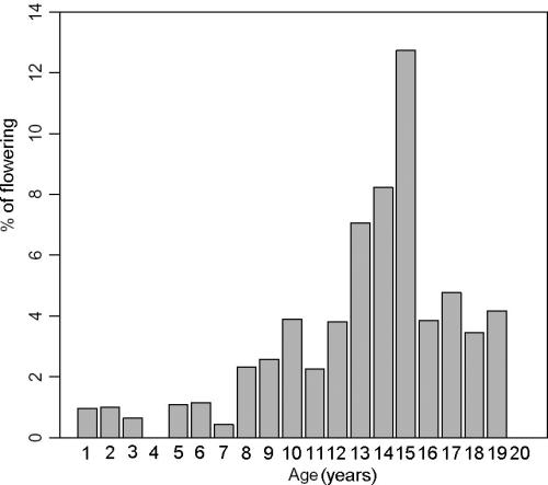
Inflorescence frequency (IF) per age of shoots.
The boxplots analysis showed that annual vertical growth, rhizome production and leaf production generally declined in median and variance values as shoot age increased (Fig. 4). On the contrary, variability throughout the years showed an increase in the most recent lepidochronological years and interannual median fluctuations in all the time series (Fig. 5). Such pattern suggested that shoot age and lepidochronological year exerted some effect on growth and should therefore be taken into account as potential covariates when investigating the effect of flowering on growth performances.
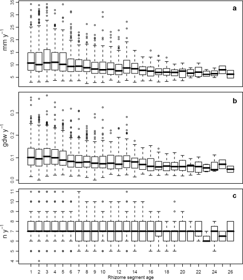
Rhizome elongation (mm year−1) (a), production (g dw year−1) (b) and leaf production (no. leaves year−1) (c) across shoot age.
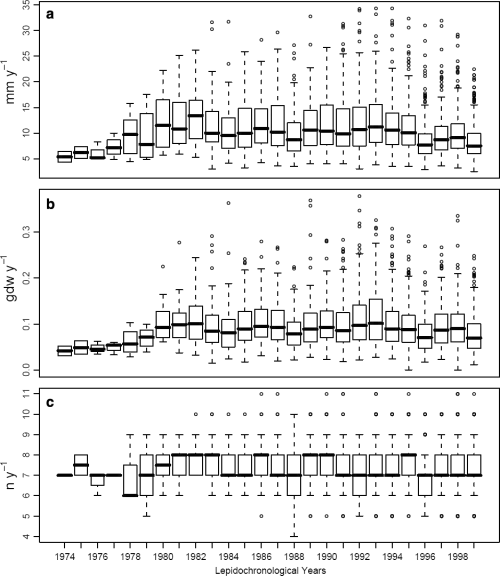
Rhizome elongation (a), production (b) and leaf production (c) across lepidochronological years.
As for the effects of flowering on growth, boxplots showed that in the year t of flowering, the median of annual rhizome elongation for flowered shoots (10 mm) was slightly higher than that for non-flowered ones (9.3 mm), while the medians for shoots which flowered 1 (t − 1) and 2 (t − 2) years before (6.0 mm, 7.0 mm, respectively) were clearly lower than those for shoots which did not flower (8.4 mm, 8.1 mm, respectively) (Fig. 6a). Similar results were detected for rhizome annual production (Fig. 6b). Again, in the flowering year t, the median for flowered shoots (0.093 g dw) was slightly higher than that for non-flowered shoots (0.089 g dw). Instead, the median production for shoots which flowered 1 year before (t − 1) was clearly lower (0.059 g dw) than that for shoots which did not flower (0.082 g dw). The difference between the medians for shoots flowering and those not flowering 2 years before (t − 2) was still negative but of smaller magnitude (0.070 and 0.074 g dw, respectively). As for leaf production, the only clear pattern was observable in the same flowering year t, when the flowering shoots produced one leaf more than the shoots which did not flower (median number of leaves for flowered shoots: 8; median number of leaves for non-flowered shoots: 7) (Fig. 6c).
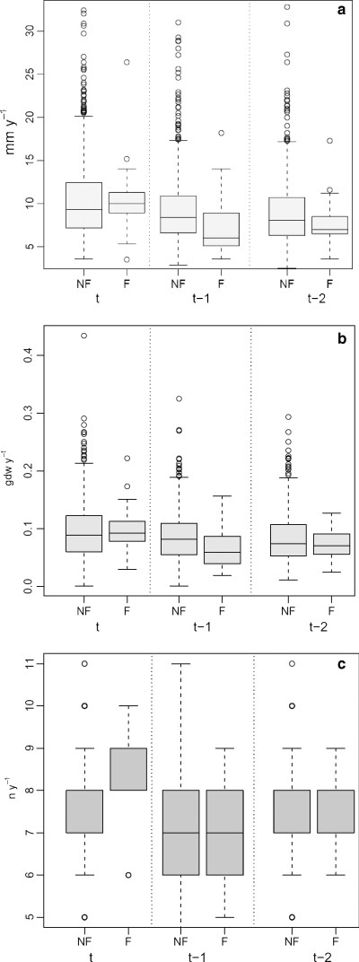
Boxplots of rhizome elongation (mm year−1) (a), rhizome production (g dw year−1) (b), leaf production (no. leaves year−1) (c) in a given year t, for shoots with (F) and without (NF) flowering, when flowering occurred in the same year t, 1 (t − 1) and 2 years (t − 2) before the year t.
For the purpose of building up the statistical GLMM, it must be underlined that only 14 lepidochronological years (from 1986 to 1999) were retained. The years before 1986 were omitted as the number of shoots with such long series of lepidochronological data was limited (Fig. 2), and this circumstance could have endangered the power of statistical inferences. Furthermore, no flowering episodes were observed before 1986 (Fig. 2). Therefore, including the 1974–1985 period would have simply worsened imbalance between flowered and non-flowered shoots, without providing further information on the issue under investigation.
The intercept (Marzamemi site) estimated for vertical growth (Table 1) was 19.7 mm year−1 (P < 0.001). The effect of flowering in the year t was moderately positive on rhizome elongation during the same year (1.5 mm year−1; P = 0.0796), whilst it has significant negative lagged effects. Namely, we observed that a shoot flowering at time t − 1 on average showed in the year t a decrease in rhizome elongation of about 15% compared with the values of the rhizomes that did not flower (−3 mm year−1; P < 0.001). The negative effect of flowering on growth persists for the two following years, as indicated by the significance of the explanatory variable ‘flowering at time t − 2’ (−2.4 mm year−1; P < 0.001). Such an effect is anyway weaker than it is in the year t − 1, and it disappears completely if we try to include furtherly lagged effects in the model. Highly significant differences between shoots within site [SD  = 0.24 log (mm year−1); P < 0.001] and negative effects of shoot age (−0.4 mm year−1; P < 0.001) and lepidochronological year (−0.4 mm year−1; P < 0.001) were observed. The sites Ognina Bay and Cape Passero showed statistical differences from the Marzamemi site.
 indicates the heterogeneity among shoots within sites. Significance codes: ***P < 0.001; **P < 0.01; *P < 0.05; †P < 0.1; ‡P < 1.
| explanatory variables | effect | t-ratios | P-value | |
|---|---|---|---|---|
| log(mm year−1) | mm year−1 | |||
| intercept | 2.98 (0.048) | 19.7 | 62.266 | <2e-16*** |
SD  |
0.24 (0.006) | – | 41.501 | <2e-16*** |
| flower t | +0.07 (0.041) | +1.5 | 1.754 | 0.0796† |
| flower t − 1 | −0.17 (0.041) | −3 | −4.046 | 5.73e-05*** |
| flower t − 2 | −0.13 (0.061) | −2.4 | −2.105 | 0.035* |
| age | −0.02 (0.002) | −0.4 | −13.84 | <2e-16*** |
| lepidochronological year | −0.02 (0.002) | −0.4 | −10.343 | <2e-16*** |
| Cape Negro | −0.03 (0.019) | −0.5 | −1.375 | 0.169† |
| Ognina Bay | +0.05 (0.019) | +1 | 2.691 | 0.007** |
| Cape Passero | −0.15 (0.02) | −2.7 | −7.473 | 1.08e-13*** |
Rhizome production (Table 2) at time t was not influenced by a flowering occurring in the same year, whereas a negative effect of flowering was observed in the two next years: it was stronger for shoots at time t − 1 (reduction by 25%) and weaker for shoots at time t − 2 (reduction by 13.3%). Moreover, as further time lags did not help to better explain the interannual production variation, they were not used in the model. Cape Negro and Ognina Bay showed significant differences from the intercept whilst significant heterogeneity among shoots within site and negative effect of shoot age were observed; no effect of lepidochronological year was noticed.
| explanatory variables | effect | t-ratios | P-value | |
|---|---|---|---|---|
| log(g dw year−1) | g dw year−1 | |||
| intercept | −2.282 (0.057) | 0.102 | −39.768 | <2e-16*** |
SD  |
0.267 (0.006) | – | 42.498 | <2e-16*** |
| flower t | +0.029 (0.049) | +0.0030 | 0.443 | 0.658‡ |
| flower t − 1 | −0.288 (0.05) | −0.0255 | −5.795 | 7.68e-09*** |
| flower t − 2 | −0.143 (0.074) | −0.0136 | −1.945 | 0.052† |
| age | −0.038 (0.002) | −0.0038 | −20.388 | <2e-16*** |
| lepidochronological year | +0.003 (0.002) | +0.0003 | 1.253 | 0.211‡ |
| Cape Negro | +0.135 (0.022) | +0.0147 | 6.039 | 1.78e-09*** |
| Ognina Bay | +0.045 (0.023) | +0.0047 | 1.998 | 0.046* |
| Cape Passero | −0.04 (0.024) | −0.0040 | −1.683 | 0.093† |
Finally, as for leaf production (Table 3), the only significant effect of flowering was that rhizomes which flowered at time t produced on average – in the same year – 0.7 more leaf than the rhizomes which did not flower. Flowering does not seem to have long-lasting effects on leaf production, as including the flowering related to the previous years in the model did not give any significant contribution. Significant differences were detected among sites, while no effect of lepidochronological year and no considerable heterogeneity among shoots within individual site were observed. The only significant negative effect was related to age.
| explanatory variables | effect | t-ratios | P-value | |
|---|---|---|---|---|
| log(no. leaves year−1) | no. leaves year−1 | |||
| intercept | 2.007 (0.049) | 7.4 | 42.139 | <2e-16*** |
SD  |
0.001 (0.006) | – | 0.022 | 0.983‡ |
| flower t | +0.088 (0.044) | +0.68 | 1.974 | 0.048* |
| age | −0.004 (0.001) | −0.03 | −3.049 | 0.002** |
| lepidochronological year | −0.001 (0.002) | −0.01 | −0.458 | 0.647‡ |
| Cape Negro | +0.0497 (0.02) | +0.37 | 2.511 | 0.012* |
| Ognina Bay | +0.0288 (0.02) | +0.21 | 1.435 | 0.151‡ |
| Cape Passero | +0.035 (0.02) | +0.27 | 1.71 | 0.088† |
Discussion
Most of the flowering events occurred in a few lepidochronological years (1987, 1995, 1998), reaching a maximum FI in 1998; this result confirms both the direct observations carried out in 1998 describing an unusual massive fruiting occurred in the area (Di Martino 1999) and the indirect findings obtained by lepidochronological analysis along the coast off Sardinia (Buia et al. 2005). Several authors reported reproductive events in 1995 in most of the meadows of the Mediterranean Sea (Acunto et al. 1996; Bussotti & Guidetti 1996; Stoppelli & Peirano 1996; Bussotti et al. 1998; Sandmeier et al. 1999; Balestri & Cinelli 2003; Balestri & Vallerini 2003; Balestri 2004), corroborating the hypothesis that P. oceanica is inclined to bloom simultaneously in the whole basin (Pergent & Pergent-Martini 1990). In most of the years none or a few flowering episodes are recorded. Hence, as it is confirmed by other studies (Pergent et al. 1989; Pergent & Pergent-Martini 1990; Bussotti & Guidetti 1996; Balestri & Vallerini 2003; Diaz-Almela et al. 2006), P. oceanica is a plant that flowers at ‘clusters’ in time. It can be noted that flowering occurred annually from 1997 to 1999 in the south-eastern Sicilian coast, as observed by Buia & Mazzella (1991) and by Balestri & Cinelli (2003) in other areas.
Moreover, it can be observed a monotonic increase in the flowering probability with age up to a certain level, followed by a clear decrease at the older ages. The maximum IF per age occurs, in fact, at the age of 15 years, ageing point at which the IF trend starts a clear decline. This pattern partially confirms the conclusions in the study by Balestri & Vallerini (2003), although in that case the decline of the flowering probability occurs in shoots older than 6 years. On the contrary, our observations are not in agreement with those reported by Diaz-Almela et al. (2006), showing an exponential increase in flowering probability with shoot aging. These variable results suggest the existence of different thresholds of the IF distributions across age between different geographic areas in the Mediterranean Sea.
As to the statistical modelling analysis, the GLMM turned out to be a suitable tool for handling spatio-temporal biological and ecological records. More specifically, this model included all the features of the data isolating the flowering effect on growth performances from effects attributable to age, time and site. In line with other studies, shoot age has a significant negative effect on rhizome elongation (Pergent & Pergent-Martini 1990) and it is quantitatively consistent with the effect estimated by Tomasello (2005) and Tomasello et al. (2005), while the decline due to lepidochronological year might be due to interannual environmental modification affecting rhizomes (Marbà & Duarte 1997). Thus, if we leave out the changes in variability mentioned above and in this paper considered as biases, flowering exerts a twofold effect: an improvement in P. oceanica growth performances (leaf production and rhizome elongation) during the flowering episodes followed by a relatively strong decline of production and elongation. Contrary to the study by Balestri & Vallerini (2003), our results suggest that flowering stimulates shoot growth in the year of the reproductive event and it produces a lagged depressing effect (at least 2 years after flowering) on rhizome elongation and production. Other lagged effects were undetectable to the model chosen for the analysis.
According to the model estimate, approximately one leaf more is produced by shoots during the sexual reproductive event, thus confirming the higher number of leaves found by Pergent (1987) on flowering shoots. The short-term increase in leaf production is probably related to the additional carbon demand required for inflorescence elaboration (Gobert et al. 2005) and seed production.
Rhizome elongation shows a synchronous response with leaf production during the flowering years. The existence of a close (1:1) relationship between leaves, production of rhizome internodes and the reiterative modality of shoots growth (Duarte et al. 1994) could explain the moderate increment in rhizome elongation here observed. On the contrary, the lack of fluctuations in leaf production for the two subsequent years conflicts with the strong negative variation affecting rhizome growth, leading us to examine other explanations. Given the elongation and production estimated by the model, we calculated that the impacts of the reproductive event in terms of loss in growth performance are about 15% and 25%, respectively, for the first year subsequent to the flowering. Such variation range is similar to that showed by Buia et al. (2005), where a decrease of 18% of rhizome growth rate in flowered shoots was observed.
Moreover, as the flowering effect persists for the two years following the sexual event and assuming that these could be combined, we altogether calculated that the impact of flowering in terms of loss in rhizome elongation and production are about 27% and 38%, respectively.
Such a considerable value could explain the very low probability of a shoot blooming again within 2 years after the first reproductive episode, as also reported by Pergent et al. (1989) and Balestri & Vallerini (2003).
Comparing the flowering effect (−27% and −38%) with annual decrease due to ageing (−2.2% and −3.7%), we concluded that the flowering impact is approximately equivalent to 10–12 years ageing (Tables 1 and 2). Hence, if a 19-year-old shoot (representing the maximum shoot age of flowering recorded –Fig. 3) switches from vegetative growth to sexual reproduction, it will experience a global stress equivalent to becoming 31–33 years old in the following two years, or a loss of about 120% and 70%, respectively, in rhizome production and elongation.
Although it has been demonstrated that time recovery to the stress induced by sexual reproduction is relatively limited (2 years), the reproductive cost for a large seagrass species like P. oceanica may become quite considerable if compared with the whole lifespan of shoots (Duarte 1991). According to our calculations, it is possible that the cost associated with sexual reproduction could be difficult to bear for shoots with greater age, suggesting that the species capacity to regulate the internal resource economy (Buia et al. 2005) could be limited by other physiological stresses linked to ageing.
Acknowledgements
This paper is dedicated to the memory of Lucia Mazzella, whose studies on the Mediterranean seagrasses and their reproductive phenology contributed significantly to the development of knowledge about these important coastal marine ecosystems. We wish to acknowledge the anonymous reviewers and the editors for their very helpful comments and fruitful suggestions. We thank also Filippo Luzzu and Antonino Scannavino for their help in SCUBA diving and support to our field activities, Vito Muggeo for his help with statistical graphics in R and Carmelo Donato for correcting grammatical and spelling mistakes. This work was supported by grants from the MIUR (Cluster 10 – Ambiente Marino – progetto n. 6; P.R.I.N. Cofin. 2004 ‘Trattamento statistico della complessità e dell'incertezza negli studi ambientali’).


