No-analog climates and shifting realized niches during the late quaternary: implications for 21st-century predictions by species distribution models
Abstract
Empirically derived species distributions models (SDMs) are increasingly relied upon to forecast species vulnerabilities to future climate change. However, many of the assumptions of SDMs may be violated when they are used to project species distributions across significant climate change events. In particular, SDM's in theory assume stable fundamental niches, but in practice, they assume stable realized niches. The assumption of a fixed realized niche relative to climate variables remains unlikely for various reasons, particularly if novel future climates open up currently unavailable portions of species’ fundamental niches. To demonstrate this effect, we compare the climate distributions for fossil-pollen data from 21 to 15 ka bp (relying on paleoclimate simulations) when communities and climates with no modern analog were common across North America to observed modern pollen assemblages. We test how well SDMs are able to project 20th century pollen-based taxon distributions with models calibrated using data from 21 to 15 ka. We find that taxa which were abundant in areas with no-analog late glacial climates, such as Fraxinus, Ostrya/Carpinus and Ulmus, substantially shifted their realized niches from the late glacial period to present. SDMs for these taxa had low predictive accuracy when projected to modern climates despite demonstrating high predictive accuracy for late glacial pollen distributions. For other taxa, e.g. Quercus, Picea, Pinus strobus, had relatively stable realized niches and models for these taxa tended to have higher predictive accuracy when projected to present. Our findings reinforce the point that a realized niche at any one time often represents only a subset of the climate conditions in which a taxon can persist. Projections from SDMs into future climate conditions that are based solely on contemporary realized distributions are potentially misleading for assessing the vulnerability of species to future climate change.
Introduction
Given the projections of extensive future climate changes (IPCC, 2007), it is important to understand how species are likely to respond (Dawson et al., 2011). Statistical species distribution models (SDMs) have been one of the most common tools employed to forecast species range shifts and potential biodiversity losses (Thuiller, 2004; Stralberg et al., 2009). These models typically correlate the observed presence or abundance of a species with environmental variables and use these correlations to predict across space and time. SDMs have been shown to have high predictive accuracy when predicting the current distributions of species across many taxa and regions of the world (Elith et al., 2006), and their relative simplicity means that future predictions can be rapidly completed for large numbers of taxa (e.g. Engler et al., 2011). However, SDMs make important assumptions about the relationship between species distributions and their environment (Wiens et al., 2009) that may limit their ability to accurately predict future species distributions.
The theoretic underpinning for SDMs is the Grinnellian/Hutchinsonian concept of species niches, in which multiple environmental factors jointly limit the geographic distribution of species (Chase & Leibold, 2003; Colwell & Rangel, 2009). Originally, Hutchinson (1957) distinguished a fundamental niche (the total range of environmental conditions in which positive population growth could be maintained) from a species’ realized niche (the environmental conditions actually occupied), and invoked biotic interactions as the primary reason why a species-realized niche might be less than its fundamental niche. However, two other sets of mechanisms may also prevent a species from fully occupying its fundamental niche: (1) dispersal limitation preventing some organisms from occupying suitable habitats, and (2) the extension of a species fundamental niche beyond the range of realized environments at a moment in time (Jackson & Overpeck, 2000). Hence, we follow Colwell & Rangel (2009)'s recommended usage of realized niche as any reprojection of a species distribution from geographic coordinates to climatic coordinates, without reference to the particular mechanism that limits a species fundamental niche.
Crucially, the calibration of statistical SDMs is based on the observed realized niche, and so their future predictions will be accurate only if fundamental niches are stable within a species (Huntley et al., 1989; Pearman et al., 2008a), and the mechanisms causing the realized niche to differ from the fundamental niche are also stable throughout its range and across time. Unfortunately, these assumptions may prove unwarranted, given the evidence for within-species adaptation to local environments, rapid evolution of invasive species to new environments (Sexton et al., 2002; Dlugosch & Parker, 2008), and the likelihood that rapid climate change will increase the importance of dispersal limitations on species ranges (Loarie et al., 2009).
Future climates with no modern analog pose a particularly acute challenge for statistical SDMs (Williams & Jackson, 2007; Williams et al., 2007), because many species probably have truncated niches, i.e. fundamental niches that extend beyond the limit of current climatic conditions (Feeley & Silman, 2010). For these species, empirically calibrated niche models would tend to incorrectly predict that a species cannot tolerate future conditions that exceed the current observed limits (Feeley & Silman, 2010). Assessing whether and how far species’ fundamental niches extend into portions of climate space not observed at present is a major challenge both for ecologists seeking to assess the threats to biodiversity posed by warmer-than-present future climates (Colwell et al., 2008; Deutsch et al., 2008; Feeley & Silman, 2010) and for Quaternary scientists seeking to draw inferences about past environments from paleoecological data (Gonzales et al., 2009).
Two avenues exist to test the predictive skill of SDMs for no-analog environments: predicting the distributions of invasive species in their new habitats (Fitzpatrick et al., 2007; Broennimann & Guisan, 2008) and hindcasting species distributions using historic and paleoecologic data (Martinez-Meyer et al., 2004; Pearman et al., 2008b). The predictive accuracy of SDMs for invasive species has often been low, perhaps because biotic interactions may limit the distributions of invasive species in their native ranges, whereas environmental factors more strongly limit their distributions in invaded ranges (Duncan et al., 2009). In addition, invasive species can exhibit rapid trait evolution in their invaded range (Sexton et al., 2002; Dlugosch & Parker, 2008). In some cases, when SDMs are used to project from native to invaded range or vice versa, species are found to occupy distinct environmental conditions in each region, suggesting either evolutionary adaptation or a release from constraints in their native range (Broennimann et al., 2007; Fitzpatrick et al., 2007).
Studies that employ a historic approach – i.e. calibrating models under present climate conditions and then hindcasting or vice versa – have shown moderately accurate predictive skill for projecting 20th-century changes in the distribution of birds (Araújo et al., 2005), plants (Dobrowski et al., 2011), and insects (Kharouba et al., 2009). However, the rate and magnitude of 20th century climate change is small relative to the changes projected for the 21st century (IPCC, 2007) or those during the last deglaciation (Jackson & Overpeck, 2000). Many studies have attempted to hindcast predictions for late-Quaternary climates, but a large proportion of these studies did not provide an independent validation of their predictions (occurrence data from both time periods) or were limited to isolated time windows, specifically full-glacial (21 ka bp) and mid-Holocene (6 ka bp) climates (Nogúes-Bravo, 2009). During the late Quaternary, climates with no modern analog were most common in unglaciated North America between 17 and 8 ka, due to changes in insolation, ice extent, and CO2 concentrations (Williams & Jackson, 2007; Roberts & Hamann, 2012). These past no-analog climates provide an underexploited opportunity to test the ability of SDMs to project the distributions of taxa across novel climates.
Studies modeling invasive species and those hindcasting to historic conditions have both found that species may have shifted their realized niches in response to new environmental conditions (Broennimann et al., 2007; Pearman et al., 2008b). Niche stability and hence the prediction accuracy of SDMs across time may be linked to species traits. Pearman et al. (2008b) found that species which were competitively dominant for light were more likely to have stably realized climatic niches during the last 6000 years and were modeled more accurately across time. Dobrowski et al. (2011) found higher accuracy for projecting SDMs across 20th century climate change in wind dispersed plants than plants that used other dispersal strategies, suggesting that species with better dispersal abilities are better able to track optimal climate conditions. Briles et al. (2011) found that the community composition of shrub and tree taxa that grew on ultramafic soils remained relatively unchanged despite the dramatic climate change events of the last deglaciation, whereas the composition of nonultramafic tree taxa changed in association with climate. This evidence suggests that there may be tradeoffs between species traits and either broad or narrow climatic tolerances.
Herein, we use fossil-pollen datasets from eastern North America in combination with paleoclimate simulations to explore the stability of species–climate relationships during past periods of no-analog climates and the implications of instability for the predictive ability of SDMs. Some plant taxa show apparently large differences between their realized niches at present vs. their distributions for the late Pleistocene and early Holocene. We also employ randomization tests of the observed pollen abundance in environmental space (Broennimann et al., in press) to quantitate the apparent shifts in realized niches and examine variations among taxa and taxa grouped into broad functional types. We then test how well SDMs calibrated with data for 21 to 15 ka bp can predict contemporary plant distributions and validate the predictions against datasets of modern pollen abundances and distributions.
Materials and methods
Pollen data
Fossil pollen relative abundance data were derived from eastern North America sites in the Neotoma paleoecology database (www.neotomadb.org) supplemented by contributions from individual researchers. All sites have updated age models, with biostratigraphic ages from well-dated sites used as new chronological controls to constrain the age models at other sites (Blois et al., 2011). Site age models were recalibrated using clam (Blaauw, 2010) and standardized to IntCal09 (Reimer et al., 2009). The revised age models for all sites have been archived at www.neotomadb.org. Cross-validation analyses of the biostratigraphic ages suggest a temporal uncertainty on the order of 500 years (and is much lower for individual well-dated sites), making this dataset suitable for the millennial-scale analyses pursued here.
The pollen dataset only included taxa resolvable at least to genus (with a few exceptions for palynologically indistinguishable genera such as Ostrya/Carpinus), and taxonomy was consistent across sites. Relative abundances of pollen types in each sample were calculated relative to the sum of all upland pollen types; we subsequently disregarded taxa found at only a few sites. The relative abundance of each taxon at each site was linearly interpolated between samples to 1 kyr intervals, and was never temporally extrapolated beyond the limits of the available age controls. As the pollen types used here are readily identified by palynologists, absences are true absences, and so, the number of samples for each taxon within a time period is equal for all taxa although some taxa are more abundant than others. Given that many prior studies have shown that pollen relative abundances are a good proxy for plant relative abundances (e.g. Delcourt et al., 1984; Paciorek & Mclachlan, 2009), yet directly modeling the pollen-to-vegetation relationship remains a major computational challenge (Sugita, 2007a,b; Paciorek & Mclachlan, 2009), here we work directly with the pollen relative abundance data.
Climate data
Climate data were derived from two recent general circulation models (GCMs), a transient version of the CCSM3 model (Liu et al., 2009) and Hadley Centre general circulation model (HadCM3) (Singarayer & Valdes, 2010). Both GCMs are based on physical models of the atmosphere and are independent of fossil-pollen data. CCSM3, however, was run forward in a transient mode with prescribed boundary conditions continuously evolving from an initial state at 22 ka bp, whereas HadCM3 was run for a series of equilibrium snapshots spaced 1000 years apart, beginning at 120 ka bp. At the time of this analysis, the highest-resolution data available from the CCSM3 simulation archives were decadal averages of seasonal variables, and so, seasonal variables were used from both GCMs. For each millennium between 21 and 0 ka bp, decadal averages of seasonal climate variables from the first 100 years of the climate simulations were extracted and averaged (e.g. 21.0–20.9 ka bp, etc.). Centennial summaries were used, so that paleo SDMs could be compared with modern observed climate that are also available at centennial scales. Note that there is a slight mismatch between the centennial resolution of the climate data and the temporal resolution of the pollen data, because the pollen data are represented by point-scale interpolations of relative abundance. However, because of temporal uncertainties in the age models of the pollen data, the pollen abundances are effectively point-scale estimates with a centennial-scale uncertainty, and so, on average, they have a centennial-scale resolution. Hence, this mismatch should not greatly affect the analyses done here.
Variables used for modeling included mean daily maximum and mean minimum temperature and mean monthly precipitation for each season: December–February (DJF), March–May (MAM), June–August (JJA) and September–November (SON). In addition, several bioclimatic indices were derived from the GCM outputs and used for modeling: the mean diurnal range (mean of seasonal (maximum temperature – minimum temperature)), temperature seasonality (intraannual standard deviation of mean seasonal temperatures*100), temperature seasonal range (maximum temperature of the warmest season -minimum temperature of the coldest season), and precipitation seasonality (intraannual coefficient of variation among seasons) (Hijmans et al., 2005).
The climate data from both GCMs were statistically downscaled and debiased following the standard change–factor approach (Wilby et al., 2004). For each climate variable at each 1000-year time interval, the difference between modeled paleo-climate and modeled modern climate was calculated. This anomaly was then resampled to a 0.5 × 0.5 degrees grid to match the resolution of the observed CRU climate dataset for 1900–1999 (Mitchell & Jones, 2005, http://badc.nerc.ac.uk/view/badc.nerc.ac.uk__ATOM__dataent_1256223773328276, accessed 4/23/2011) using bilinear interpolation. The resulting downscaled anomaly was then added to the observed modern CRU dataset to produce the downscaled and debiased paleoclimate at 0.5 × 0.5 degree resolution. Modern pollen data were attributed with climate data from the CRU dataset. In all cases, climate maps were clipped to the region represented by a minimum convex polygon with a 100-km buffer surrounding the locations of pollen samples for the given time period.
Species distribution models
There are many different algorithms available for modeling species distributions (Elith et al., 2006). We used five different modeling algorithms to correlate the relative abundance of each pollen taxon with environmental variables: boosted regression trees (BRT, Elith et al., 2008), multivariate adaptive regression splines (MARS, Leathwick et al., 2006), a multi-response version of MARS (MARS-COM, Elith & Leathwick, 2007), generalized additive models (GAM, Hastie & Tibshirani, 1990), and generalized linear models (GLM, McCullagh & Nelder, 1989). Detailed descriptions of each of the algorithms can be found in the references, and specific settings as applied to this study can be found in Supplementary Information 1. Recently, several studies have argued that because a significant proportion of variation in future climate models is due to the algorithm chosen (Diniz-Filho et al., 2009), ensembles from multiple algorithms may produce more accurate future models (Araújo & New, 2006). To compensate for this potential source of uncertainty, we also created two ensemble models to test whether ensembles of algorithms and climate models predict better than any single algorithm or GCM. The first ensemble was created by taking a weighted average of the predictions across all algorithms for each GCM, where weights are based on the mean cross-validated deviance from models from the calibration time period. The second ensemble used the weighted average across all algorithms and GCMs.
The climatic variables included in the SDMs varied across taxa. We examined scatter plots of the abundance of each taxon vs. each climate variable using data pooled from 21 ka bp to 15 ka bp to identify variables that may limit the distribution and abundance of each taxon. Climate variables that exhibited a potential correlation in the scatter plots were chosen for inclusion in the models. We also used the scatter plots to identify the form of the relationship for GLMs (linear or quadratic). No other model selection was performed.
To examine the predictive ability of SDMs across time periods with significant climate change, models were calibrated with a pooled dataset from 21 ka bp to 15 ka bp years ago and then applied to predict contemporary species distributions (modern pollen samples). Using multiple time periods in the calibration dataset increases the likelihood of capturing a species’ fundamental niche (Nogúes-Bravo et al., 2008; Nogúes-Bravo, 2009), and here includes taxon distributions for both the cold/dry climates of the last glacial maximum and the more-seasonal-than-present temperatures of the late glacial period (Kutzbach et al., 1998; Williams & Jackson, 2007). SDM predictive ability across time was evaluated by seeing how well projections fit the relative pollen abundances for 0 ka. Predictive ability was evaluated using the correlation between observed and predicted relative pollen abundance. We also used a 10-fold cross-validation of the pollen data from within the model calibration time period as an estimate of within-time prediction accuracy, following approaches widely used to evaluate contemporary simulations with SDMs (Fielding & Bell, 1997). The data were randomly split into 10 equal-sized groups. Models were iteratively calibrated with nine of the groups, and predictions were tested with the remaining held-out group. The average cross-validated estimate of predictive accuracy was compared with the actual predictive accuracy to modern data to assess how well within-time cross-validation estimates true predictive skill across time periods of major climatic change.
We ran two additional analyses to test the predictive skill of models calibrated from other time periods. First, we ran a series of SDMs simulations in which we expanded the initial 21 to 15 ka bp calibration dataset by iteratively adding data from each successive 1 ka interval and predicting models to 0 ka. Second, we created models from each millennium from 14 ka bp to 1 ka bp and predicted to 0 ka. These two analyses can identify times when the past realized niches of taxa become more or less similar to late-Holocene realized niches and can illustrate whether pooling data across time improves predictive skill.
Quantitating climatic niche shifts
We used a new method for quantitating the similarity of realized niches across time that is designed to allow comparisons even when the background environmental conditions differ. We extend the methods of Broennimann et al. (in press) to test for the equivalence and similarity of the abundance of pollen for each taxon in relation to the environmental space occupied by a taxon from two time periods. The method uses a principal components analysis (PCA) based on climate data from all nonglaciated grid cells in the analysis area. The PCA is calculated on a matrix where rows are grid cells from the climate data, and each column is a different climate variable. The late glacial (21 to 15 ka bp) and modern climate data are combined in the matrix, and the rows are weighted by the number of grid cells in each respective time period. Pollen abundances for each taxon were then plotted in a two-dimensional environmental space created from the first two principal components using thin plate spline spatial interpolation of the observed pollen sites. The 2-D environmental space was clipped, so that only the points that occurred in both periods were used to assess niche overlap to limit the effects of extrapolations of the thin plate splines. The overlap of interpolated pollen abundance between the two time periods was evaluated using Schoener's D, an index of niche overlap that has been used in conjunction with SDMs (Warren et al., 2008). Schoener's D varies between 0 and 1, with 0 indicating no niche overlap and 1 indicating identical niches.
We used two randomization tests to test for niche equivalence and niche similarity across time for each taxon (Warren et al., 2008, Broennimann et al. in press). Niche equivalence was assessed by comparing the overlap from the same taxon at time 1 and time 2 to the niche overlap based on two pseudo taxa. The pseudo taxa are created by randomly polling the observed data from the taxon at time 1 and time 2, but maintaining the sample sizes of each time period. The null hypothesis is that the observed overlap is indistinguishable from the overlap based on randomly pooled data. A significant result indicates two taxa that do not have equivalent realized niches. The second test asks if the realized niche of a taxon in one time is more (or less) similar to abundance values randomly assigned to PCA coordinates drawn from the background climate data of the other time period. The null hypothesis is that the observed niche overlap is no different from the overlap of a taxon randomly assigned to the climate space of the other time period. A significant result indicates overlap in realized niches that is more similar or less similar than the overlap with the randomly created taxon. Significant results for the niche similarity test indicate that the observed pattern has a signal of niche similarity that is detectable while accounting for the similarity in background climates between the two time periods. The niche similarity test was run in both directions, e.g., random taxon created using modern climate and random taxon created using late glacial climate. For both tests, 100 random pseudo taxa were created per taxon.
To see if groups of vegetation type were more or less likely to have stable realized niches across time, each taxon was grouped into broad plant functional types following Williams et al. (2004); needle-leaved woody (Pinus strobus, Tsuga, Abies, Picea), herbaceous/small shrub (Cyperaceae, Artemisia, Ambrosia, Poaceae), broad-leaved woody (Betula, Quercus, Alnus, Fagus, Salix, Acer, Carya), and no-analog broad-leaved woody. The no-analog broad-leaved woody class comprises Fraxinus, Ostrya/Carpinus, Ulmus, and Populus taxa that are known to have peak abundances during the late glacial no-analog climates (Jacobson et al., 1987; Williams & Jackson, 2007). Niche overlap (D) and SDM predictive model accuracy were summarized by plant functional type for each millennium between 15 ka bp and 1 ka bp (15 ka bp represents data pooled from 21 ka bp to 15 ka bp).
Results
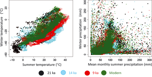
Plots of the CCSM3-simulated climate space across time show that some past climates have no current analog, and that some portions of climate space, which existed in the past, have disappeared over time (Fig. 1). The most striking signal is the appearance of high-seasonality temperatures during the late Pleistocene and early Holocene, caused by higher-than-present seasonality of insolation (Williams & Jackson, 2007) and lower-than-present CO2. This is most strongly expressed at 14 ka bp when the simulated climate indicates a large portion of North America that included climates with more seasonal temperature than during any other period over the last 21 ka (Fig. 1a). The climate space that includes modern summer and winter temperatures is a subset of earlier time periods, whereas areas of climate without current analog occur in each of the other time periods (Fig. 1a). As climate warmed during the late Pleistocene, large regions of climate space disappeared from North America, particularly regions with the coldest winter and summer temperatures (lower left corner of Fig. 1a). As opposed to temperature, the simulated precipitation across North America has been relatively stable in climate space during the last 21 ka (Fig. 1b).
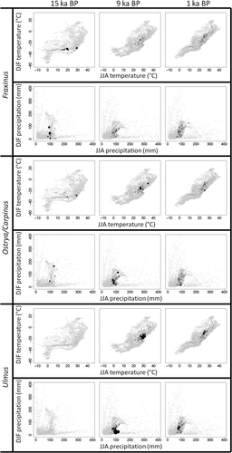
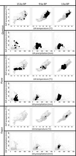
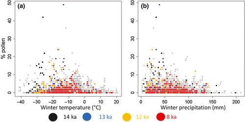
Some taxa apparently had relatively stable climatic distributions through time, whereas others show apparent shifts that we illustrate using with plots of pollen abundance in relation to winter and summer temperature and precipitation, climate variables that typically represent extreme conditions likely to constrain the distribution, and abundance of species in Eastern North America (examples shown in Figs 2 and 3). For some taxa, the regions of climate space with peak pollen abundance have shifted through time (Fig. 2). The highest pollen abundance for both Fraxinus and Ostrya/Carpinus occurred in areas with more seasonal temperature 14 ka bp than at 9 or 1 ka (Fig. 2), whereas Ulmus had higher pollen abundance in areas with wetter summers and dryer winters at 9 ka bp compared with the pollen abundance recorded from 1 ka bp. Fraxinus pollen abundances plotted against summer temperature and winter precipitation highlights the large shifts in the climatic distributions of this taxon over time (Fig. 4). Between 14 and 8 ka bp, the maximum abundances declined and the position of the mode shifted toward wetter and warmer climates (Fig. 4). In contrast, the distribution of Quercus, Picea, and Fagus pollen abundance in climate space is relatively stable through time (Fig. 3).
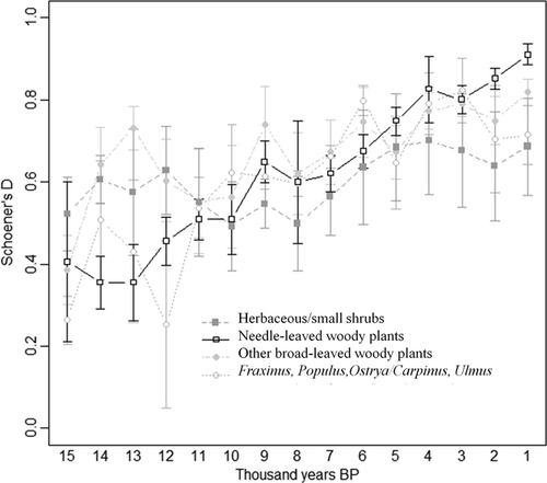
The niche overlap analyses as measured by Schoener's D reveals that shifts in the patterns of pollen abundance relative to climates through time were common across the 20 taxa studied here (Table 1, Data S2). We fail to reject the null hypothesis of niche equivalency in only 30% of the taxa analyzed, meaning that, for 70% of taxa, we reject the null hypothesis that taxa have equivalent realized niches across time (Table 1). Tests of niche similarity for late glacial models predicting modern pollen abundances found that only 20% of taxa were more similar than would be expected than taxa created at random from modern climate, 50% of the taxa were less similar than random and in 30% of taxa we failed to reject the null hypothesis (Table 1) . For 11 of the 20 taxa, the result of the similarity test changed depending on which time period used real data and which time period was used to randomly select data (Table 1). Across all functional types, the temporal trends in the similarity of realized niches closely tracked the similarity of overall climate (Fig. 5): when climate was more similar to present, realized niches were more similar to present. This suggests that the emergence of no analog climates in the past was a first-order driver of the observed shifts in realized niches. For broad-leaved woody plants, niche overlap increased from 15 ka bp to 13 ka bp and then decreased around 12 ka bp, a period during which climate rapidly returned to near-glacial conditions following the end of the Bølling-Allerød and the onset of the Younger Dryas. No-analog broad-leaved woody plants (Fraxinus, Ostrya/Carpinus, Ulmus, and Populus) exhibited a similar pattern, but niche overlap was substantially less than other broad-leaved woody plants for the period 15 ka bp to 12 ka bp. In contrast, needle-leaved woody taxa exhibited increasing niche overlap with their modern climatic niche through this time period (Fig. 5). Herbaceous plants and small shrubs generally exhibited the most stable realized climatic niches through time. From 6 ka bp to present, the niche overlap with modern realized niches stabilized for all functional types except needle-leaved taxa, whereas the niche overlap with modern niches continued to increase for needle-leaved taxa through 1 ka bp (Fig. 5).
| Taxon | Overlap | Equivalence test | Similarity test | Similarity test |
|---|---|---|---|---|
| D | P | P (LGM–modern) | P (Modern–LGM) | |
| Betula | 0.61 | 0.02 | 0.14 | 0.97 |
| Quercus | 0.51 | 0.02 | 0.02 † | 0.02 * |
| Alnus | 0.33 | 0.02 | 0.04 † | 0.06 |
| Cyperaceae | 0.51 | 0.02 | 0.99 | 0.02 † |
| Pinus strobus | 0.13 | 0.02 | 0.02 † | 0.38 |
| Artemisia | 0.58 | 0.48 | 0.73 | 0.02 * |
| Tsuga | 0.013 | 0.02 | 0.02 † | 0.14 |
| Ambrosia | 0.41 | 0.02 | 0.02 † | 0.89 |
| Ulmus | 0.29 | 0.02 | 0.02 † | 0.29 |
| Fagus | 0.1 | 0.02 | 0.02 † | 0.02 † |
| Fraxinus | 0.2 | 0.02 | 0.5 | 0.12 |
| Salix | 0.29 | 0.02 | 0.02 * | 0.04 † |
| Abies | 0.74 | 0.38 | 0.02 * | 0.02 * |
| Asteroideae | 0.29 | 0.02 | 0.02 † | 0.06 |
| Ostrya/Carpinus | 0.21 | 0.02 | 0.02 † | 0.02 † |
| Acer | 0.16 | 0.02 | 0.02 † | 0.08 |
| Populus | 0.38 | 0.06 | 0.09 | 0.28 |
| Carya | 0.8 | 0.48 | 0.02 * | 0.02 * |
| Poaceae | 0.82 | 0.06 | 0.69 | 0.04 * |
| Picea | 0.74 | 0.06 | 0.02 * | 0.02 * |
- If the P < 0.05, the tests indicate that the observed overlap is greater than the overlap between real and random taxa (*), or that the overlap is less than the overlap between real and random taxa (†). In all cases, bolded entries are significant.
Distributional model predictive accuracy
We found considerable differences in the predictive accuracy of late glacial SDMs (calibrated with data from 21 to15 ka bp), predicting modern pollen abundance among the taxa studied from the different modeling algorithms and GCMs tested (Data S1). However, when predictive accuracy was evaluated across all models, there was no statistical difference in the predictive accuracy from the different algorithms or GCMs (Data S1), indicating that no algorithm or GCM consistently outperformed another. Similarly, ensembles of the different algorithms and ensembles of algorithms and GCMs were no better at predicting modern pollen abundance than individual algorithms. We ranked individual algorithms by the number of times each had the highest predictive accuracy per taxon for each GCM. Boosted regression trees (BRT) models ranked highest, along with generalized linear models (GLM) and multivariate adaptive regression splines (MARS), but prediction accuracy was more consistent across GCMs for BRT models (Data S1). The CCSM3 GCM was ranked highest of the GCMs for 10 of the 20 taxa, the Hadley model was highest for 9 of the 20, and the ensemble of all algorithms and both GCMs ranked highest for one of the 20 taxa (Data S1). For simplicity, the remainder of the SDM results and niche overlap analyses are reported for BRT models using the CCSM3 GCM, which performed best based on our rankings.
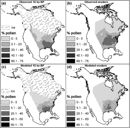
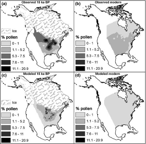
A direct consequence of the intertaxonomic differences in the stability of climatic distributions (Figs 2 and 3) is that the accuracy of predictions by species distribution models (when calibrated with data from 21 to15 ka bp) varied considerably among taxa. For example, the boosted-regression tree models for Quercus accurately predicted the 21 to 15 ka bp pollen distribution with a cross-validated correlation of 0.79 between observed and predicted pollen relative abundance. When the model was projected to modern climates, the accuracy declined, with a correlation of 0.470, but the overall spatial patterns in Quercus pollen abundance were accurately predicted (Fig. 6). For other taxa, models had high within-time cross-validation accuracy, but were unable to accurately predict modern distributions. The models for Fraxinus produced accurately reproduced pollen distribution for 21 to 15 ka bp (cross-validation correlation: 0.64), but projected an almost complete absence of Fraxinus at present despite regions in the upper Midwest of the United States that have moderate observed pollen abundances (correlation between predicted and observed distribution for modern: −0.17; Fig. 7).
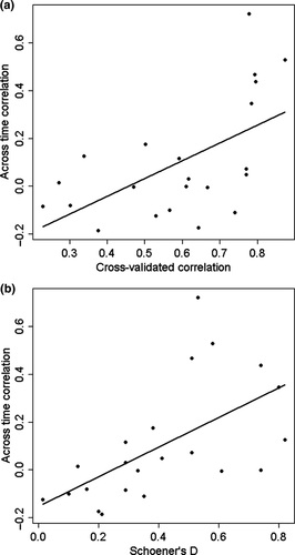
Across all taxa, SDM projections to 0 ka were consistently less accurate than the estimated cross-validated accuracy for 21 to 15 ka bp (Fig. 8a). However, we found a significant linear regression of cross-validated correlation vs. across time correlation (slope = 0.75, P = 0.005, r2 = 0.34), indicating that models with higher within-time cross-validated accuracy had higher across-time accuracy. A linear regression of across-time accuracy (Fig. 8b) vs. Schoener's D (Fig. 5) indicates that taxa with higher realized niche overlap across time also had the greatest predictive accuracy when projections were made to modern climate (Fig. 8b, slope = 0.62, P = 0.004, r2 = 0.35).
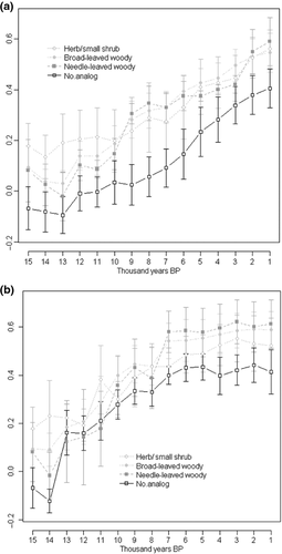
Our SDM analyses in which we expanded the calibration dataset by iteratively adding data from successive 1 ka time periods indicated an increase in predictive accuracy for all functional types as the calibration data set was augmented through time (Fig. 9a). Abrupt transitions from lower to higher predictive accuracy occurred when 12 ka bp was added to the calibration data set for all functional types except herbaceous and small shrubs. For broad-leaved woody and needle-leaved woody taxa, another abrupt improvement in prediction accuracy was found when 9 ka bp was added to the calibration data set (Fig. 9a). When models were calibrated with data from each individual millennium, prediction accuracy increases from 21–15 ka bp to 7 ka bp, but then does not improve from 7 ka bp to 1 ka bp for all life forms (Fig. 9b). Similarly, the relative ranking of the predictive accuracy for each of the life forms changes between successive millenniums up until 7 ka bp at which point the rankings do not change through 1 ka bp (Fig. 9b).
Discussion
Combining fossil-pollen data with paleoclimate simulations spanning the last deglaciation suggests that some taxa have occupied distinct realized niches at different points in time, partially in response to past climates unlike any at present. Previous work has shown that species have responded individualistically to Quaternary climate changes by shifting their geographic distributions to track favorable conditions (Davis, 1981; Huntley & Birks, 1983; Prentice et al., 1991). Our work suggests that for some taxa, these shifts in geographic distribution through time were accompanied by shifts in their climatic distribution (Fig. 2). This pattern is most pronounced for periods of no-analog climates, i.e. climates outside modern North American climate space (Figs 1-4).
The causes of these realized niche shifts need further study, but there are three overarching and nonexclusive possibilities. First, these analyses are based on overlaying fossil-pollen datasets on paleoclimatic simulations, and so, realized niche shifts may be in part due to errors in the data and models. However, errors in the data and climate simulations are unlikely to completely explain this phenomenon, because the realized niche shifts are consistent with prior knowledge about the patterns and drivers of late-Quaternary climate and vegetation changes. The emergence of no-analog climates in the past, characterized by a higher-than-present thermal seasonality, is consistent with orbital forcing that caused higher-than-present insolation seasonality in the Northern Hemisphere (Kutzbach et al., 1998; Williams et al., 2001). Initial data-model comparisons for CCSM3 indicate that these simulations reproduce major features of the evolution of the climate system between 22 and 14 ka bp, including time series of surface air temperatures over Greenland and Antarctica, Atlantic sea-surface temperatures, and rates of Atlantic meridional oceanic circulation (Liu et al., 2009). In addition, our results do not change significantly when we use the HadUM simulations.
The pollen datasets are the latest iteration of sites underlying the well-documented shifts in late-Quaternary vegetation distributions, and significantly improve upon previous datasets of fossil-pollen data from eastern North America (Davis, 1981; Jacobson et al., 1987; Webb et al., 1993; Williams et al., 2004). The revised pollen data are updated to the latest calibration curve (IntCal09; Reimer et al. 2009) and systematically deal with potential age model error due to bulk sediment dates (Grimm & Jacobson, 2003). The temporal uncertainty in this dataset is roughly 500 years for the late Pleistocene, and is much lower for some sites and times (Blois et al., 2011). Most of our tests are based on models calibrated with data pooled from 21 to 15 ka, prior to the period of large millennial-scale fluctuations in the climate system. For this time period, multi-centennial temporal uncertainty in the pollen data is unlikely to cause large mismatches to the climate data.
Another potential concern is that we are largely working with genus-level data, and so, the observed shifts in niches may be due to different species becoming more or less abundant at different points in time. It is unlikely that the genus-level changes in niche space that we find are largely due to species extinctions, as there is only one documented case of a plant species going extinct during the late Quaternary in North America (Jackson & Weng, 1999). Still, given the data at hand, we cannot distinguish the niche space occupied by different species within a genus during this period. Even so, this begs the question of why the abundances of these species are changing over time: the realized niche for a genus will shift if and only if one or more of its constituent species experience a shift in its realized niches. For example, the key species of Fraxinus in the late glacial no-analog communities is probably F. nigra (Cushing, 1967; Grimm & Jacobson, 2003), which is widespread at present across northeastern North America. So, F. nigra is a species that was widespread both in the past and at present, and yet, the genus-level realized niche of Fraxinus – based on its fossil-pollen distribution – is completely different (Fig. 4), suggesting that F. nigra has gone from being a relatively abundant species under highly seasonal climates in the past, to a common but more minor constituent of the modern flora. In addition, there is ample evidence for significant variations in the realized niches of populations within a species (Garzón et al., 2011), and so, the problem of within-taxon variations in climatic tolerances for genus-level vs. species-level is more a problem of degree rather than kind.
The second possible cause for the observed realized niche shifts are that the observed shifts could represent evolutionary alterations in species fundamental niches, caused by adaptations to late-Quaternary climate change. Recent studies have shown the ability of some species to adapt to rapid changes in environmental conditions (Dlugosch & Parker, 2008). We cannot rule out the possibility that similar kinds of evolutionary adaptations occurred during the last 20,000 years (Davis et al., 2005). However, the oscillation in Schoener's D between 15 and 12 ka bp (Fig. 5) shows that all taxa alternated between having more and less similar realized niches to present, during a period of rapid climate change in the Northern Hemisphere (Fig. 5). It seems somewhat unlikely that species evolved in response to warming during Bølling-Allerød warming and developed fundamental niches more similar to present, then evolved yet again to cooling during the Younger Dryas, and then again as climate warmed in the early Holocene.
The third possibility, which we regard as the most probable, is that these results are caused by shifts in realized niches within a larger, possibly stable, fundamental niche that is truncated at present by the finite domain of contemporary climates (Williams & Jackson, 2007; Nogúes-Bravo, 2009; Feeley & Silman, 2010). The observed realized niche shifts are consistent with the hypothesis that some taxa have truncated climatic niches during periods that correspond with no-analog climates. For example, both Fraxinus and Ostrya/Carpinus show high pollen abundances in regions of environmental space at 15 ka bp that do not occur under modern climates (Fig. 2). Similarly, taxa that are associated with no-analog climates exhibit the greatest differences in realized niche position relative to modern climate from 15 ka bp to 8 ka bp (Fig. 4). No-analog climates open regions of climate space that some taxa may be preadapted to exploit, resulting in shifting realized niches. Many plant populations exhibit considerable phenotypic plasticity with regard to climatic limits to distribution and abundance which allows them to adapt rapidly to climate change without requiring the evolution of their fundamental niche (Nicotra et al., 2010). Furthermore, the individualistic responses of plant taxa to past climate changes resulted in mixtures of species with no modern analog (Williams et al., 2001). These would have produced novel species interactions, which may have shifted the distributions of relative abundances for individual taxa along climatic gradients.
A useful future research direction would be to examine if particular species traits offer some explanation for whether species have stable or labile realized niches through time . In studies of the recent past, the distributions of species with greater dispersal ability have been modeled more accurately across time suggesting that these species are better able to track favorable conditions and may imply that a trade-off exists where greater dispersal ability may come at the cost of lower niche breadth (Dobrowski et al., 2011). Recent work has shown that the taxa adapted to ultramafic substrates in the Siskiyou mountains exhibited stable pollen percentages during the last 15 thousand years, whereas the abundance of taxa on nonultramafic substrates in the region varied considerably through time (Briles et al., 2011). Similarly, grassland communities adapted to low-productivity edaphic conditions showed smaller responses to experimental warming than grassland communities in high-productive edaphic conditions (Grime et al., 2008). Uncovering the traits which are more likely to be correlated with stable realized niches would help with identifying which taxa are better suited for climate-impact predictions by SDMs. Our results are not explicitly tied to species traits; however, we do find that among the plant life forms we compared, needle-leaved taxa are the only group that continued to increase the overlap in past realized niches with present niches throughout the study period, whereas niche overlap for other life forms was stable from 6 ka bp through 1 ka bp (Fig. 5). This result suggests that needle-leaved taxa, which tend to be more tolerant to cold climates, have taken the longest to reach a climatic equilibrium following the last deglaciation, and that these taxa may still not have reached an equilibrium with current climate. The observed pattern for other life forms never reaching complete overlap with modern niches may be due to nonclimatic factors, for example, anthropogenic alterations to the landscape may be preventing modern taxa from occupying all suitable climatic conditions.
Whatever the explanation for the observed shifts in realized niches, they result in poor SDM predictive accuracy when models are projected across times that encompass major climate change. Declines in accuracy were most pronounced for taxa that occupied no-analog climate conditions of the past. Cross-validation analyses for a single time period did provide a predictive metric of future performance, but one that consistently overestimated future predictive ability (Fig. 8).
Our results show that taxa often do not occupy their entire fundamental niche in any one period and that different regions of the fundamental niche are realized at different points in time. Thus, calibrating SDMs based upon a single time period can cause a species fundamental niche to be incompletely represented, and predicted future distributions may be overly restricted (Nogúes-Bravo, 2009). These findings suggest considerable caution while interpreting the results of models when projections are made across time periods with significant climatic differences. The truncation of species fundamental niches by contemporary climates is a major source of uncertainty when projecting ecological responses to future climate change (Wiens et al., 2009; Feeley & Silman, 2010), and one likely to produce surprising ecological responses to future novel environments (Williams & Jackson, 2007).
Our results suggest that, for many plant taxa, the large climate-driven shifts in geographic ranges during the late Quaternary were accompanied by substantial shifts in realized climatic niches. The strengths of these shifts varied among taxa, and are most pronounced for plant taxa with peak pollen abundances during late glacial climates with no modern analog. Shifts in plant distributions along climatic axes are interpreted as shifts in species realized niches, as taxa expanded into portions of their fundamental niche that is not available at present. However, the possibility cannot be ruled out that these shifts are due in part to evolutionary adaption and shifts in species’ fundamental niches. Regardless of the cause, the apparent shifts in taxon-climate relationships strongly reduce the predictive ability of SDMs. Within-time period cross-validation analyses can indicate which taxa will be better predicted in the future, but generally provide inflated estimates of SDM predictive skill. Although these analyses are limited to the late Quaternary, they suggest caution in over-interpreting SDM projections for future climate change, and also suggest that we may be underestimating the climatic tolerances of species when using modern-only calibration datasets.
Acknowledgements
This work was supported by the Climate, People, and Environment Program at the Nelson Institute Center for Climatic Research at the University of Wisconsin, the Focus on Energy Environmental and Economic Research Program, and the National Science Foundation (EAR-0844223). This work was improved by discussions with David Nogués-Bravo, Simon Brewer, Carsten Rahbek, Jason McLachlan, Mark Vellend, and Heather Kharouba. This is CCR Publication Number 1011.


