Fixing a snag in carbon emissions estimates from wildfires
[Correction added on 18 July 2019 after first online publication: The values in the final sentence of the Abstract have been corrected.]
Abstract
Wildfire is an essential earth-system process, impacting ecosystem processes and the carbon cycle. Forest fires are becoming more frequent and severe, yet gaps exist in the modeling of fire on vegetation and carbon dynamics. Strategies for reducing carbon dioxide (CO2) emissions from wildfires include increasing tree harvest, largely based on the public assumption that fires burn live forests to the ground, despite observations indicating that less than 5% of mature tree biomass is actually consumed. This misconception is also reflected though excessive combustion of live trees in models. Here, we show that regional emissions estimates using widely implemented combustion coefficients are 59%–83% higher than emissions based on field observations. Using unique field datasets from before and after wildfires and an improved ecosystem model, we provide strong evidence that these large overestimates can be reduced by using realistic biomass combustion factors and by accurately quantifying biomass in standing dead trees that decompose over decades to centuries after fire (“snags”). Most model development focuses on area burned; our results reveal that accurately representing combustion is also essential for quantifying fire impacts on ecosystems. Using our improvements, we find that western US forest fires have emitted 851 ± 228 Tg CO2 (~half of alternative estimates) over the last 17 years, which is minor compared to 16,200 Tg CO2 from fossil fuels across the region.
1 INTRODUCTION
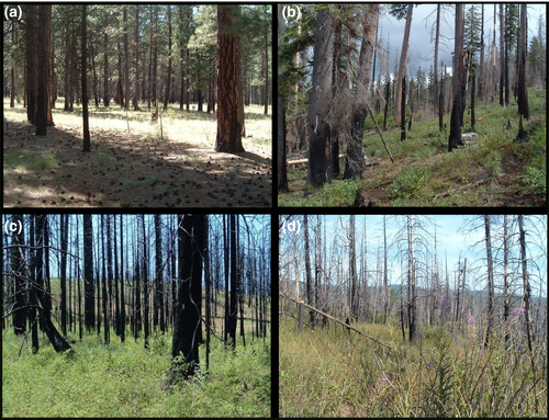
Temperate forests of the western United States are significant carbon stocks (Buotte et al., 2019; Pan et al., 2011) and include some of the most carbon-dense forests on Earth (Hudiburg et al., 2009). Increasing forest fire activity threatens these carbon stores in parts of the region because larger burn areas can lead to more tree mortality (Abatzoglou & Williams, 2016; Hicke, Meddens, & Kolden, 2016; Westerling, Hidalgo, Cayan, & Swetnam, 2006). However, contemporary CO2 emissions to the atmosphere from fire are often significantly exaggerated because of public and policymaker misconceptions that forests commonly “burn to the ground” during fire and that mortality equals emissions (Figure 1) (Mater, 2017; Zinke, 2018). The reality is instead negligible stem combustion of live, mature trees (i.e., <5%; Figure 2), followed by gradual decomposition over years to centuries (Campbell, Donato, Azuma, & Law, 2007; Law & Waring, 2015). Modeled estimates of fire emissions reinforce public misconceptions, as tree mortality is often mistranslated into 30%–80% of tree carbon emitted immediately (van der Werf et al., 2010; Wiedinmyer & Neff, 2007), and is in conflict with observations (Lutz et al., 2017). It is important to rectify overestimates because governments are currently using mortality and emissions estimates from fire to inform land management decisions intended to mitigate climate change (California, Executive Department, 2018; Fears & Eilperin, 2019; Nunez, 2006; Oregon, 2005; UNFCCC, 2015; U.S. Executive Office of the President, 2018), emphasizing the need for model improvement using field observations.
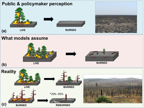
While modeling research focuses primarily on improving representation of area burned due to the availability of validating satellite products (Hantson et al., 2016; Thonicke et al., 2010), it is critical to recognize that simulations can generate inaccurate estimates of combustion dynamics through a combination of (a) unrealistic combustion coefficients (i.e., the biomass fraction that burns) and (b) misrepresentation of forest biomass (i.e., carbon) pools. Models use assumed fractions of biomass combusted (combustion coefficients) in fire and apply that to the biomass in the area burned. These default combustion coefficients overestimate pool combustion when they exceed ranges of observed combustion across live and dead pools, effectively simulating events where forests “burn to the ground.”
The largest discrepancies between modeled and observed combustion of aboveground biomass exist for live, mature trees, which are the dominant pool of aboveground carbon across western US forests (Ghimire, Williams, Collatz, & Vanderhoof, 2012; Hudiburg et al., 2009; Wilson, Woodall, & Griffith, 2013). Default values for live tree bole (stem) combustion can range from 30%–80% (S1 and S2) in high-severity events, but post-fire observations in the western United States indicate actual combustion is nearly nonexistent for mature trees in fire-prone ecosystems (Campbell, Alberti, Martin, & Law, 2009; Campbell, Fontaine, & Donato, 2016; Lutz et al., 2017). Field experiments show that there is inadequate prolonged heat to facilitate combustion of live tree stems, even at the highest fire intensities (Smith et al., 2016; Sparks et al., 2017).
Most models also lack standing dead tree carbon pools (snags; Table S2), essential for representation of forests in the context of disturbance and mortality (Edburg et al., 2012). High-severity fires can kill live trees, which become snags and the dominant stock of aboveground carbon in burned areas (Campbell et al., 2007; Figures 1d and 2). When trees die in a “no snag” model, the wood instead transfers to the forest floor, becoming downed-woody debris (Figure 1c). In drier climates, snags decompose at slower rates than downed-woody debris (Wirth, Gleixner, & Heimann, 2009), producing relatively slow emissions over decades rather than acute, large pulses through combustion. Further, biomass location matters for reburn combustion (Campbell et al., 2007; Ghimire et al., 2012); simulating snags as downed-woody debris facilitates higher rates of combustion in subsequent fires.
Generally, model fire severity is defined by the amount of biomass killed and consumed. Representation of combustion in models varies from a single severity (“static severity,” e.g., CLM 5.0; Lawrence et al., 2018) to a range from low-to-high (“variable severity,” e.g., LANDIS-II; Sturtevant, Scheller, Miranda, Shinneman, & Syphard, 2009; Table 1, and Tables S1 and S2). These dynamic coefficients are either “categorical” or calculated through fire submodels that largely depend on fuel moisture and tree or woody debris size class (Table S2). Default mortality and combustion coefficients can be “parameterized” to be more in line with observations; however, this is often not done, especially at large scales (Buotte et al., 2019; Liang, Hurteau, & Westerling, 2018; Tables S6, S7, and S8); modeling experiments instead often rely on restricting predicted burn area or fire occurrence to achieve realistic combustion (Hudiburg, Law, & Thornton, 2013; Hudiburg, Luyssaert, Thornton, & Law, 2013). There is also large variation in the biomass pools represented, with a persistent absence of snags. Even models that include dynamic combustion coefficients (e.g., LPJ-GUESS-SPITFIRE) or variable severity (e.g., LANDIS-II) can overestimate emissions because the rate at which standing wood becomes downed wood is too high without a snag pool (Figure 1c).
|
Rim fire (YFDP) Pool |
Stock (Mg C/ha) | Combustion (%) | Model (%) (moderate-severity) |
|---|---|---|---|
| Tree | 281.3 (53.2) | 0.1 (0.0) | |
| Foliage | — | — | 80–92 |
| Branch | — | — | 30–92 |
| Bark | — | — | 30–46 |
| Bolewood | — | — | 30–46 |
| Shrub | 2.9 | 95.4 | na |
| Snag | 13.9 (3.0) | 61.5 (8.8) | na |
| Coarse woody debris | 39.5 (19.6) | 58.3 (33.5) | 28–50 |
| Fine woody debris | 3.3 (1.4) | 94.4 (5.0) | 50–100 |
| Litter | 11.9 (1.5) | 90.4 (4.8) | 50–100 |
| Duff | 43.6 (5.7) | 88.5 (4.3) | 50–100 |
| Total | 396.4 (54.4) | 21.9 (5.0) | na |
|
Biscuit fire (high-severity subset) Pool |
Stock (Mg C/ha) | Combustion (%) | Model (%) (high- severity) |
|---|---|---|---|
| Tree | 92.5 | 8.7 | |
| Foliage | 5.6 | 73.0 | 80–100 |
| Branch | 14.8 | 7.9 | 30–100 |
| Bark | 11.7 | 21.0 | 30–80 |
| Bolewood | 60.5 | 0.6 | 30–80 |
| Snag | 7.7 | 17.6 | na |
| Coarse woody debris | 7.6 | 34.1 | 28–80 |
| Fine woody debris | 1.1 | 78.0 | 50–100 |
| Litter | 9.2 | 100.0 | 50–100 |
| Duff | 6.0 | 99.0 | 50–100 |
| Total | 124.0 | 22.5 | na |
Note
- All combustion percentages are equal to combustion coefficients except for the Rim Fire snag pool, where the percentage combines combustion and transfer of snag biomass to downed-wood pools. Bold italicized numbers highlight discrepancies between the range of model coefficients (Table S6, S7, S8; Lawrence et al., 2018; Sturtevant et al., 2009) and field observations for live trees. Field observations are from this study and previous studies (Campbell et al., 2007; Lutz et al., 2012). Standard deviation of YFDP subplots shown in parentheses where applicable.
In this study, we compare a range of default combustion coefficients and forest structure representations of regional-to-global-scale models with observation-based combustion coefficients and a newly implemented model snag pool. Our observation-based refinements utilize carbon stock datasets that span fire events, including new, detailed field observations from the 2013 Rim Fire in California (Lutz et al., 2017). We also simulate post-fire carbon cycle dynamics using an improved version of the globally recognized biogeochemical model DayCent (Hudiburg, Higuera, & Hicke, 2017; Parton, Hartman, Ojima, & Schimel, 1998) through addition of snag pools with varying combustion, decomposition, and fall rates (Figure S1). We then estimate 2000–2016 fire emissions across the western United States with our improved methods.
2 MATERIALS AND METHODS
We calculated emissions from forest combustion in the western US states using site observations, the monitoring trends in burn severity (MTBS) burn perimeter database, and ecosystem modeling. Mortality and combustion coefficients were generated from plot data collected before and after fire in the region and from commonly used models. We developed a modified version of DayCent (Straube et al., 2018) that introduces a snag pool to improve representation of post-disturbance ecosystem structure and fluxes. DayCent was also used to simulate commonly used model combustion coefficients and mortality transfers in both snag-free and snag-enabled versions. Finally, we estimated recent western US forest emissions (2000–2016) for the same range of combustion and pool structures using forest inventory-derived plot biomass carbon estimates combined with the MTBS burn perimeter and severity database (Eidenshink et al., 2007).
Fire combustion coefficients from the 2013 Rim Fire were calculated using the Yosemite Forest Dynamics Plot (YFDP; CA; Lutz, Larson, Swanson, & Freund, 2012) dataset. The YFDP (37.77°N, 119.82°W) is part of the Smithsonian ForestGEO network of spatially explicit monitoring plots (Anderson-Teixeira et al., 2015). The YFDP is a carbon-dense, mixed-conifer forest, where live trees contained ~70% of aboveground biomass pre-fire (Table 1 and Table S4). The YFDP (800 m × 320 m) was divided into ten, 160 m × 160 m quadrats, and pre- and post-fire aboveground carbon pools were calculated for each quadrat (Table 1, and Tables S3 and S4). The plot was burned in an unattended backfire set by Yosemite National Park to check the advance of the Rim Fire (Lutz, Larson, & Swanson, 2018; Lutz et al., 2017).
At plot inception (2009–2010), all trees were identified, mapped, and tagged. Snags were measured as to height, diameter, top diameter, and decay class. Shrub patches were delineated as polygons and shrub biomass was calculated by plot-specific allometric equations (Lutz et al., 2014). Due to the 113 year period of fire exclusion (Barth, Larson, & Lutz, 2015), herbaceous cover was de minimus. Each pre-fire year (2011–2013), trees were visited to ascertain their status in May–June, and therefore, the 2013 survey provided a comprehensive inventory of standing stems. In May 2014, we performed the post-fire survey, noting tree death, whether tree canopies were scorched or combusted, and measuring dimensions of partially combusted snags.
In 2011 and 2014, surface fuels were measured with 1,600 m transects following the methods of (Brown, 1974) with additional data taken on large woody debris (1,000 hr fuels, ≥10 cm diameter). Live biomass was calculated using the methods of Chojnacky, Heath, and Jenkins (2013). Snag biomass was calculated using the same equations as when trees were killed by fire when needles were only scorched. Pre-fire biomass of snags was calculated as the mass of the bole only, calculated as a conic frustum.
Combustion estimates were also used from published studies in mature Oregon forests. (Campbell et al., 2007, 2016; Meigs, Donato, Campbell, Martin, & Law, 2009; Figure 2; Table 1). Observations from the 2002 Biscuit Fire showed that live tree combustion was limited primarily to canopy combustion and bark scorching, resulting in a maximum 7% mature tree combustion at high (stand-replacing) severity. These datasets also contained reburned plots that burned 15 years earlier in the 1987 Silver Fire. The authors did not find any significant differences between the combustion coefficients of the aboveground pools in the reburn versus the initial burn; however, because significantly more of the carbon was in snag, downed wood, or small diameter tree pools, more aboveground carbon did combust.
Simulations were performed using a modified version (developed by the authors) of the biogeochemical model DayCent (Chen et al., 2016; Straube et al., 2018) that introduces standing dead pools and fluxes. DayCent is the daily time step of CENTURY, simulating fluxes of carbon and nitrogen between the atmosphere, ecosystem, and soil (for further model description see Figure S1). Our modified DayCent now incorporates standing dead pools of leaves, fine branches, and large wood into the forest submodel, as well as accompanying fluxes of carbon and nitrogen involved in both background senescence and prescribed fire and harvest events (Figure S1). Fluxes in and out of standing dead pools are governed by inputs from death of live pools, fall rates of standing dead material, decomposition, photodegradation, and removal by harvest or fire. Attached dead leaves that fall to the ground are partitioned into surface structural and metabolic litter. When standing dead wood falls, it becomes coarse and fine woody debris. Live and dead material involved in fire events may now be returned to the system as charcoal.
Simulations were performed for each of the combustion and mortality parameter sets (Table S5) extracted from the YFDP 2013 Rim Fire, 2002 Oregon Biscuit Fire, and additional regional datasets of partial aboveground combustion (e.g., Fahnestock & Agee, 1983; Kauffman & Martin, 1989; Knapp, Keeley, Ballenger, & Brennan, 2005; Meigs et al., 2009). DayCent pre-fire carbon pools and fluxes were parameterized to the 2011 and 2013 carbon stocks of the YFDP (Table 1, and Tables S3 and S4; Lutz et al., 2012). Model spinup (2,000 years) was based on a pre-modern fire return interval of 29 years followed by 120 years of no fire, consistent with historical park records. Site soil characteristics were extracted from SSURGO (NRCS, 2010). Site climate (temperature and precipitation) was based on location data from PRISM (Daly, Taylor, & Gibson, 1997) for 1981–2017. Post-fire simulation periods in model experiments were driven with historical climate conditions. Mortality proportions were based on fire severity mortality classes (Campbell et al., 2016; Meigs et al., 2009) comparable to the mortality in the “variable-severity” model (below), facilitating comparison. Mortality classes include 0%–10%, 10%–50%, 50%–90%, and 90%–100% for very low-, low-, moderate-, and high-severity fire, respectively.
DayCent was also used to simulate default parameter sets from the Community Land Model v 5.0 (CLM; Lawrence et al., 2018; Oleson et al., 2013) and LANDIS-II with the Net Ecosystem Carbon and Nitrogen Succession (NECN) and Dynamic Fuels & Fire System (Sturtevant et al., 2009) (Scheller et al., 2007) (Tables S6, S7, and S8). These two models represent the range of coefficients and severities used by most other fire-enabled ecosystem, forest landscape, and dynamic vegetation models (Tables S1 and S2). In our results, CLM and LANDIS-II default parameters, respectively, inform our “static” and “variable” severity scenarios (combustion and mortality). In total, we performed 18 scenario simulations of the YFDP representing the range of fire severity, pool combustion, and mortality transfer assumption scenarios.
CLM is the land model of the Community Earth System Model (CESM) and simulates the fluxes of energy, water, chemical elements, and trace gases between atmosphere, plants, and soil. As the land-model component of CESM, CLM is a globally utilized model in the effort to explore land-climate feedbacks, and has been used to research forest–climate interactions throughout the western United States (Buotte et al., 2019; Hudiburg, Law, et al., 2013; Hudiburg, Luyssaert, et al., 2013). During fire events, CLM employs single severity and mortality. Combustion is therefore governed by burn area. CLM first combusts litter, coarse woody debris, and live trees, and then transfers non-burned tree biomass to dead pools (Table S8).
LANDIS-II is a forest landscape model simulating growth and succession of tree species and age cohorts. LANDIS-II with NECN (derived from CENTURY/DayCent) is used to explore the potential effects of evolving climate, disturbance regimes, and management on ecosystem structure and composition. During a grid cell fire event, species cohort mortality is determined as a product of fire severity and species tolerance, with up to 100% of species cohorts killed and mortality occurring as death of all cohorts below a variable percentage of species longevity. Fire reduction parameters determine emissions and specify reduction of dead wood and litter after the above mortality scheme kills and deposits biomass on the forest floor in the same time step (Tables S6 and S7). We calculated LANDIS-II equivalent biomass mortality estimates for the YFDP dominant stand species (White fir and Sugar pine).
Western US carbon stocks were calculated from over 80,000 forest inventory plots (FIA) containing over 2.5 million tree records in the region following methods developed in previous studies (Hudiburg et al., 2009; Hudiburg, Law, Wirth, & Luyssaert, 2011; Law et al., 2018; Law, Hudiburg, & Luyssaert, 2013). Uncertainty estimates for total regional emissions were calculated using a propagation of error approach accounting for error in biomass allometrics and the MTBS fire perimeters (Law et al., 2018).
Western US fire emissions were calculated from 2000 to 2016 using MTBS (Eidenshink et al., 2007) estimates of burn area and severity combined with FIA plot biomass data aggregated by ecoregion and forest type (30 m pixel resolution; Table S9) and severity-specific combustion factors for each pool (large stems, small stems, downed dead wood, understory, standing dead, litter pools (Campbell et al., 2007; Meigs et al., 2009; and Rim Fire values from this study). Areas of recurring severe fire based on the MTBS record (less than 2% of total burn area included reburns from 1984 to 2016; Table S10) were combusted with modified biomass pools reflecting simulated post-fire conditions using combustion observations from reburned plots in the Biscuit Fire study (Campbell et al., 2007, 2016; Donato, Fontaine, & Campbell, 2016). Combustion factor scenarios were consistent with DayCent YFDP simulation sets by carbon pool (see Tables S5–S8). Observation-based and the variable-severity model-based sets were applied by severity. The static-severity model combustion percentages were applied across all severities within burn perimeters. Comparisons with fossil fuel emissions were done using Environmental Protection Agency state CO2 emissions data (EPA, 2018).
3 RESULTS AND DISCUSSION
3.1 Fire emissions in carbon-dense forests
The YFDP experienced a mixed-severity burn in 2013, consuming 22% of aboveground carbon, with dead biomass producing 95% of estimated emissions (Table 1). The fire induced ~71% tree mortality (stems ≥1 cm dbh) within 1 year and combusted <1% of live tree biomass. When YFDP carbon stocks burned under the range of model scenarios, default variable and static-severity model coefficients resulted in up to 285% and 486% overestimated fire CO2 emissions compared to observation-based coefficients, respectively (Figure 3a). Overestimation resulted primarily from high default bole combustion coefficients combined with existing high live biomass. High-severity fire consumed 31% and 81% (70 and 183 Mg C/ha) of aboveground live tree carbon in model scenarios, compared to 6% (14 Mg C/ha) in the observation-based scenario.
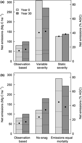
Observation-based combustion of aboveground carbon decreased from 22% (80 Mg C/ha) to 6% (22 Mg C/ha) from high- to very low-fire severity, reflecting transitions between canopy and ground fire. With variable-severity model coefficients, aboveground carbon combustion decreased from a maximum of 87% to a minimum of 10%. This wide range is explained by large modeled decreases in emissions with decreasing burn severity, averaging 20% of aboveground carbon per severity class (Figure 3a; dotted lines). By contrast, observation-based changes in emitted aboveground carbon averaged 5% per severity class. The static-severity model simulation overestimated observation-based emissions by 59%–486% (high-low observed severity).
Thirty years’ post-fire, the static-severity scenario carbon losses still exceeded those from observation-based severities by 39%–1010% (Figure 3a). The difference in emissions estimates between the variable-severity model and observation-based scenarios marginally decreased over time due to a lack of remaining biomass to decompose (Figure S3). Nonetheless, the variable and static-severity models overestimated observation-based emissions by averages of 150% and 130%, demonstrating persistent unrealistic post-fire emissions over timescales relevant to greenhouse gas management. These results highlight that model estimates can both inflate fire emissions and the potential carbon benefits of severity-reduction strategies, such as thinning for fuels reduction. Further, static-severity overestimates increase dramatically at lower severities, undervaluing the persistent carbon storage capacity of forests experiencing low-severity fire.
Omission of a snag pool resulted in increased combustion of downed-woody debris (vs. snags); net fire-event carbon losses were 50%–79% greater across no-snag scenarios (Figure 3b). Without snags, fire-killed biomass was deposited on the forest floor and decomposed at a faster rate than in the snag scenarios, where large quantities of killed biomass decayed in standing dead pools before reaching the ground (Figure S1). The combined effects of altered combustion and decomposition after 30 years yielded an average doubling of simulated net emissions across severities when snags were not represented.
From low-to-high severity, “mortality = emissions” scenarios (“public perception”; Figure 1b) exceeded observation-based emissions by 140%–253% (Figure 3b); these results were similar to variable-severity scenario results (Figure 3a). At neither 30 years nor 100 years, post-fire did the “mortality = emissions” scenario emissions decrease below the observation-based scenarios. Although up to 95% mortality was implemented in the observation-based scenarios, subsequent decomposition of dead biomass was largely compensated by regrowth. These results show that simulating mortality transfers that are distinct from combustion does not simply delay these carbon losses to the future (Figures S2 and S3); greenhouse gas emissions and impacts to the atmosphere are instead markedly decreased.
3.2 Emissions impacts across western US forest fires in the 21st century
Across the western United States, observation-based combustion emissions summed to 232 ± 62 Tg C from 2000 to 2016, emitting 23% of aboveground carbon stocks within ~11 million hectares of burned area (Figures 4 and 5), in agreement with estimates for Oregon over similar time periods (Law, 2014; Meigs et al., 2009). As at smaller scales, model-based live tree combustion overestimated observation-based combustion by an order of magnitude (Figure 4), leading to regional emissions overestimates of 59% and 83%.
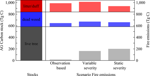
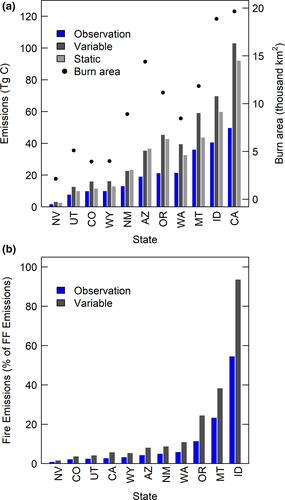
Forest fires in California, Idaho, and Montana accounted for 54% of total combustion emissions (Figure 5), resulting from higher burned area and aboveground carbon density relative to southern interior states. Coastal-state (CA, OR, WA) model-based scenarios exceeded observation-based emissions by 81% and 103%, compared to overestimates of 35% and 67% in the Northern Rockies (ID, MT, WY). This difference stemmed from greater aboveground carbon density in coastal versus Northern Rocky states. Thus, carbon loss is most overestimated in forests with high tree biomass.
Regional observation-based fire emissions totaled to 5% of fossil fuel emissions compared to twice that when using default coefficients (Figure 5b). Notably, Idaho and Montana fire emissions accounted for 55% and 24% of yearly fossil fuel emissions, respectively, highlighting the importance of correctly calculating fire emissions in the Northern Rockies due to large projected increases in fire (Westerling et al., 2006). Emissions in California and Washington were extremely low relative to fossil fuel emissions, likely because of population density (energy usage).
3.3 Implications
Our results illustrate that the use of inaccurate combustion coefficients in models can double forest fire emissions estimates across the western United States. Overestimates increase to three to four times in carbon-dense forests such as the YFDP, mostly because models incorrectly combust live trees. Treating carbon released over years to centuries as an immediate emission by equating combustion with mortality is simply inaccurate. Omitting snag representation in models compounds this error, because of altered decay and combustion dynamics.
A warming climate and more frequently recurring fire (Westerling et al., 2006) may alter some regional forest carbon stocks from the present. The field data used in this study includes area in the 2002 Biscuit Fire that contained the 1987 Silver Fire (15 years earlier), where reburned plots showed an additional 26% reduction in standing and downed dead wood due to fire compared to mature single-burn plots but similar pool combustion coefficients across fires (Donato et al., 2016). New observations from reburned lodgepole pine stands in the Greater Yellowstone Ecosystem show that young stands can lose a majority of the aboveground carbon (basal diameter <4 cm; Turner, Braziunas, Hansen, & Harvey, 2019), consistent with Biscuit Fire observations for the small conifer pool (Campbell et al., 2007). This suggests a mechanism by which recurrent burning (“reburn”) could in principle lead to state changes to treeless vegetation over the mid-term because of frequent, repeated combustion of aboveground stocks over time (Coop, Parks, McClernan, & Holsinger, 2016). The percentage of the regional forest landscape that has recently experienced such severe reburn is less than 1% (see regional methods), but could increase in the future with climate change (Dale et al., 2001; Turner et al., 2019), and disproportionally in some areas (e.g., Southern California and US Southwest). It will be essential to accurately estimate these emissions impacts in a regional context by quantifying shifting biomass pools (e.g., dead and young pools) upon which realistic combustion coefficients are applied.
Resolving modeled inaccuracies is critical because forest fire and CO2 emissions-reduction strategies are currently being implemented (California, Executive Department, 2018; U.S. Executive Office of the President, 2018). Overestimating forest fire emissions exacerbates public and policymaker misconceptions (Figure 1). Our simulations highlight the need for more studies on pre- and post-fire carbon pools over decadal durations in order to capture combustion dynamics in different forest types to provide observations for modelers to better constrain and validate their models. At present, even when models correctly estimate burned area, their ability to properly inform policy makers about the contributions of fires to greenhouse gas budgets can be inadequate, adding fuel to the fire when drafting forest management plans.
ACKNOWLEDGEMENTS
J.E.S., T.W.H., and K.J.B. were supported by National Science Foundation award number DEB-1553049 and DEB-1655183. A.M.S. and C.A.K. were supported by the National Science Foundation award DMS-1520873. A.M.S. was partially supported by the NASA Carbon Monitoring System Program Award NNH15AZ06I.
CONFLICT OF INTEREST
The authors declare no conflict of interest.


