Influence of physiological phenology on the seasonal pattern of ecosystem respiration in deciduous forests
Abstract
Understanding the environmental and biotic drivers of respiration at the ecosystem level is a prerequisite to further improve scenarios of the global carbon cycle. In this study we investigated the relevance of physiological phenology, defined as seasonal changes in plant physiological properties, for explaining the temporal dynamics of ecosystem respiration (RECO) in deciduous forests. Previous studies showed that empirical RECO models can be substantially improved by considering the biotic dependency of RECO on the short-term productivity (e.g., daily gross primary production, GPP) in addition to the well-known environmental controls of temperature and water availability. Here, we use a model-data integration approach to investigate the added value of physiological phenology, represented by the first temporal derivative of GPP, or alternatively of the fraction of absorbed photosynthetically active radiation, for modeling RECO at 19 deciduous broadleaved forests in the FLUXNET La Thuile database. The new data-oriented semiempirical model leads to an 8% decrease in root mean square error (RMSE) and a 6% increase in the modeling efficiency (EF) of modeled RECO when compared to a version of the model that does not consider the physiological phenology. The reduction of the model-observation bias occurred mainly at the monthly time scale, and in spring and summer, while a smaller reduction was observed at the annual time scale. The proposed approach did not improve the model performance at several sites, and we identified as potential causes the plant canopy heterogeneity and the use of air temperature as a driver of ecosystem respiration instead of soil temperature. However, in the majority of sites the model-error remained unchanged regardless of the driving temperature. Overall, our results point toward the potential for improving current approaches for modeling RECO in deciduous forests by including the phenological cycle of the canopy.
Introduction
The integrated respiration fluxes of terrestrial ecosystems (i.e., ‘ecosystem respiration’ RECO) represent a large flux in the global carbon cycle. Hence, to model climate–carbon cycle interactions, it is important to understand the responses of RECO to environmental conditions and biotic controls (Davidson & Janssens, 2006; Trumbore, 2006; Mahecha et al., 2010a). However, the processes and complex interactions between the different drivers controlling RECO are still not fully understood and the associated uncertainty continues to hamper bottom upscaling to regional and continental scales.
Temporal changes of RECO are partly controlled by the seasonal variability of environmental factors, in particular temperature, soil moisture or precipitation. In addition, empirical studies have demonstrated a tight link between gross primary production (GPP) and RECO for most ecosystems (e.g., Mahecha et al., 2010a; Peichl et al., 2013). These findings indicate that the seasonal variability of RECO is partially dependent on seasonal changes in the availability of new substrate produced by photosynthesis (Reichstein & Beer, 2008). Building on this idea, Migliavacca et al. (2011) showed that a significant improvement in the skill of a semiempirical RECO model (TPLinGPP) could be obtained by including GPP, along with temperature and water availability, as an additional driver. However, TPLinGPP underestimates RECO during the spring green-up (Fig. 1a and c) in deciduous forests (Migliavacca et al., 2011).
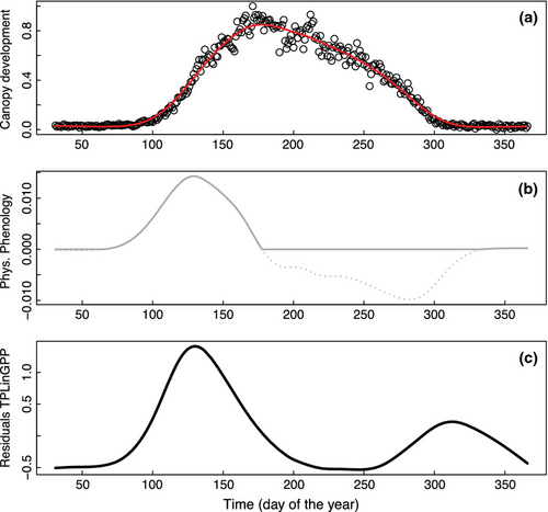
Here, we investigate the hypothesis that the bias in spring green-up is related to a peak in autotrophic respiration resulting from the intense metabolic activity during the leaf out, which was not accounted for in the TPLinGPP model. This phenomenon of seasonal changes in plant physiology is referred as ‘physiological phenology’, which extends the traditional organism-focused definition of phenology to include physiological processes (Lieth, 1974). Here, we quantify physiological phenology in terms of the first derivative of a dynamic indicator of the state of the canopy. As indicators we use GPP and the fraction of Absorbed Photosynthetically Active Radiation (fAPAR).
The rate of aboveground autotrophic respiration is influenced by foliar development because the most immediate interactions between respiration and photosynthesis occur inside the leaves (Amthor, 1994bb). Therefore, the phenology of foliar respiration typically tracks the phenology of photosynthesis (Amthor, 1994a; Ludwig et al., 1994; Law et al., 1999), except during spring green-up, when a large fraction of foliar respiration results from respiration costs associated with the construction of new leaves. Studies on several species showed that the costs of expanding buds during this period of high carbon demand are supported by carbohydrate reserves in woody tissues, rather than by photosynthetic tissue (Landhäusser, 2010; Dickmann & Kozlowski 1970). The phenology of stem respiration is synchronous to wood production which, in turn, is determined by photosynthesis (Sprugel et al., 1995; Edwards & Hanson, 1996) and temperature. The stem respiration sensitivity to temperature varies from species to species and depends on the temperature to which plants are adapted or acclimated (Korner & Larcher, 1988). Moreover, a distinct pulse in stem respiration during the spring green-up has been observed in few studies (e.g., Bolstad et al., 2004).
The influence of physiological phenology on belowground autotrophic respiration has been reported in the literature as well. Joslin et al. (2001) found a correlation between a phenology index and root elongation intensity (Wilson & Batchelard, 1975) in a mature white oak-chestnut/oak forest in Tennessee (USA). Joslin et al. (2001) further showed that factors related to phenology appeared to override environmental variables such as soil water content in controlling the root elongation rate. To explain the results, the authors referred to Hendrick & Pregitzer (1996), who showed a burst of fine root growth in early summer immediately following foliar expansion, when soil water content and temperature conditions are favorable and the supply of carbohydrates produced by the newly expanded canopy is adequate. In fact, an increasing contribution of the autotrophic root respiration to soil respiration has been observed during the spring period of root elongation and growth (Law et al., 2001; Misson et al., 2006). Other studies reported even greater increases (30–50%) in the contribution of autotrophic respiration to total soil respiration during the growing season for different temperate deciduous forests (Epron et al., 2001). Physiological phenology has been shown to control belowground respiration also through the supply of photosynthates for the respiration of roots, mycorrhiza, and heterotrophs utilizing root exudates in the rhizosphere (CurielYuste et al., 2004; DeForest et al., 2006; Davidson & Holbrook, 2009). Recently, additional insights on the seasonality of carbon cycling processes were provided by studies using radiocarbon (14C) signatures (Carbone et al., 2011). For example, Atarashi-Andoh et al. (2012) partitioned soil respiration into heterotrophic and autotrophic components using 14C signatures and an isotope mass balance approach. They found that the contribution of root-derived carbon to soil respiration in a cool-temperate deciduous forest varied according to vegetation phenology.
Because respiratory fluxes are generated by different ecosystem components, the temperature driving respiration processes might varies according to: (i) the location where they take place, and (ii) the relative importance of the aboveground (primarily driven by air temperature, TA) to belowground (primarily driven by soil temperature, TS) components (e.g., Subke & Bahn, 2010;. Therefore, the analysis of the differences and biases introduced by the choice of the driving temperature in modeling respiration is increasingly studied (e.g., Richardson et al., 2006; Lasslop et al., 2012).
The overarching objective of this study is to improve the prediction of RECO of deciduous forests during spring green-up as compared to the work of Migliavacca et al. (2011) by including a representation of physiological phenology into the TPLinGPP model. To this end we: (i) developed a modified version of TPLinGPP that includes one of two alternative proxies of physiological phenology, (ii) optimized the modified model against RECO data reported for 19 deciduous forest eddy covariance sites, (iii) analyzed the reduction of model-data bias arising from the use of physiological phenology, and (iv) evaluated model performance using alternatively soil and air temperature as drivers of respiration with the aim of quantifying the relative importance of the belowground vs. aboveground respiration components during the season.
Material and methods
The dataset
In this analysis, data from version 2 of the LaThuile FLUXNET dataset (http://www.fluxdata.org) were used. The LaThuile dataset contains 253 research sites belonging to the FLUXNET eddy covariance flux measurements network (Baldocchi, 2008). The analysis focused on 19 deciduous broadleaved forest sites (Table 1) that have at least 1 year of good quality CO2 fluxes and meteorological data (i.e., only days with <15% of gap-filled half-hours were retained), and maximum leaf area index (LAI) (Migliavacca et al., 2011).
| Site ID | Tower Name | Country | Latitude | Longitude | Climate | References |
|---|---|---|---|---|---|---|
| CA-Oas | Sask. – SSA Old Aspen | Canada | 53.63 | −106.20 | Dfc | (Black et al. 2000) |
| DE-Hai | Hainich | Germany | 51.08 | 10.45 | Cfb | (Knohl et al., 2003) |
| FR-Fon | Fontainebleau | France | 48.48 | 2.78 | Cfb | (Delpierre et al., 2009) |
| FR-Hes | Hesse Forest – Sarrebourg | France | 48.67 | 7.06 | Cfb | (Granier et al., 2000) |
| IT-LMa | La Mandria | Italy | 45.15 | 7.58 | Cfa | (Reichstein et al., 2005) |
| IT-Non | Nonantola | Italy | 44.69 | 11.09 | Cfa | (Reichstein et al., 2005) |
| IT-PT1 | Zerbolò–Parco Ticino– Canarazzo | Italy | 45.20 | 9.06 | Cfa | (Migliavacca et al., 2009) |
| IT-Ro1 | Roccarespampani 1 | Italy | 42.41 | 11.93 | Csa | (Reichstein et al., 2003) |
| IT-Ro2 | Roccarespampani 2 | Italy | 42.39 | 11.92 | Csa | (Reichstein et al., 2003) |
| UK-Ham | Hampshire | UK | 51.15 | −0.86 | Cfb | – |
| US-Bar | Bartlett Experimental Forest | USA | 44.06 | −71.29 | Dfb | (Jenkins et al., 2007) |
| US-Bn2 | Bonanza Creek, 1987 Burn site | USA | 63.92 | −145.38 | Dsc | (Liu et al., 2005) |
| US-Ha1 | Harvard Forest EMS Tower (HFR1) | USA | 42.54 | −72.17 | Dfb | (Urbanski et al. 2007) |
| US-LPH | Little Prospect Hill | USA | 42.54 | −72.18 | Dfb | (Borken et al., 2006) |
| US-MMS | Morgan Monroe State Forest | USA | 39.32 | −86.41 | Cfa | (Schmid et al., 2000) |
| US-MOz | Missouri Ozark Site | USA | 38.74 | −92.20 | Cfa | (Gu et al., 2006) |
| US-Oho | Oak Openings | USA | 41.55 | −83.84 | Dfa | (DeForest et al., 2006) |
| US-UMB | University of Michigan Biological Station | USA | 45.56 | −84.71 | Dfb | (Gough et al., 2008) |
| US-WCr | Willow Creek | USA | 45.81 | −90.08 | Dfb | (Cook et al., 2004) |
These sites are located in the Northern Hemisphere in a latitudinal range that spans from 63.92°N at the Bonanza Creek site (US-Bn2) to 38.74°N at the Missouri Ozark site (US-MOz). The climatic regions analyzed include Humid Mesothermal Climates to Humid Microthermal Climates (classes C and D), according to the Köppen classification (Peel et al., 2007).
The following daily data products of the FLUXNET dataset were used: RECO, GPP, midday net ecosystem exchange (NEE) (11:00–13:00 hours), nighttime NEE [average of half-hourly NEE selected according to a global radiation threshold of 20 Wm−2 as defined by Reichstein et al. (2005)], daily mean air temperature (TA), soil temperature (TS), and 30-day backward precipitation running average (P). At each site, flux data were storage-corrected and spike-filtered as described in Papale et al. (2006), and subsequently gap-filled and partitioned as described by Reichstein et al. (2005).
For each site, we used estimates of fAPAR, retrieved from the Sea-viewing Wide Field-of-view Sensor (SeaWiFS) following methods of Gobron et al. (2000). The validation of the Joint Research Centre (JRC) fAPAR products (hereafter referred as JRC fAPAR) is described by Gobron et al. (2006). The fAPAR used in this study covers the period from September 1997 to June 2006 with a nominal spatial resolution of 1.5 km (http://fAPAR.jrc.ec.europa.eu/) (Gobron et al., 2006). The fAPAR values correspond to the 10-day time composite products spatially averaged over 3 × 3 pixels around the tower location. For the analysis of the spatial heterogeneity of the canopy fAPAR standard spatial deviations were classified into low, medium, and high variability according to the terciles of the distributions of the spatial standard deviation of the fAPAR.
Ecosystem respiration model
Description of TPLinGPP model
 (1)
(1) (2)
(2) (3)
(3) (4)
(4)E0 (K) is the activation energy parameter and represents the sensitivity of ecosystem respiration to temperature, Tref is fixed here at 288.15 K (15 °C) and T0 is fixed at 227.13 K (−46.02 °C) (Lloyd & Taylor, 1994).
 (5)
(5)Development of the TPdGPP model
TPLinGPP was modified in the present study to reduce the spring bias observed over deciduous forests. A key insight from previous studies is that Rref can be assumed to vary during the growing season, but is dependent of specific site characteristics (Reichstein et al., 2003; Migliavacca et al., 2011), productivity (GPP, Mahecha et al., 2010a; Migliavacca et al., 2011), and physiological phenology.
The first derivative of a canopy development indicator in spring was introduced to reduce the spring bias in modeled RECO. Specifically, either GPP or fAPAR was used for this purpose, and the daily values of the first derivative of their smoothed time series (i.e., dGPP/dt and dfAPAR/dt, respectively) were computed. For this purpose the time series of daily GPP and 10-daily fAPAR were smoothed and gap-filled using a cubic spline with degrees of freedom adjusted to the length of the time series (30 for GPP and 20 for fAPAR). The first derivatives were numerically computed from the smoothed time series. Because our focus is on the spring period, we set the negative values of the first derivative that occurred in autumn to 0, retaining only values of dGPP/dt>0 (Fig. 1b).
 (6)
(6) (7)
(7)Modeling set-up
The parameters in TPLinGPP [R0, E0, α, k, and k2 in Eqns 1-5] and in TPdGPP [R0, E0, α, k, k2, and k20, in Eqn 7] were estimated for each site.
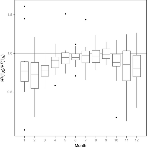
An initial analysis was conducted using the following combination of driver-observations: daily GPP, the first derivative of midday GPP, and RECO reported in the FLUXNET database (hereafter, we refer to this driver-observation set with the label GPP-dGPP-RECO). The parameters of the TPdGPP model were estimated using alternatively soil (TS) and air (TA) temperature. Then, with a moving window of 2 weeks, we computed the ratio of the coefficient of determination (R2) of the TPdGPP model simulations driven by TS to that driven by TA. The latter analysis was conducted to evaluate the ability of TS and TA in predicting RECO. When the ratio was lower than 1, a relevant contribution of aboveground respiration to the temporal variability of RECO can be hypothesized.
A second exercise was conducted using nighttime NEE in place of RECO, midday NEE (11:00–13:00 hours) in place of GPP and dfAPAR/dt as a proxy for canopy development. This analysis was conducted to confirm the results obtained with the first analysis, because GPP and RECO are partially correlated. Hereafter, we refer to this driver-observation set with the label NEEm-dfAPAR-NEEn (Table 2).
| TPdGPP | TPLinGPP | |||
|---|---|---|---|---|
| GPP-dGPP-RECO | NEEm-dfAPAR-NEEn | GPP-dGPP-RECO | NEEm-dfAPAR-NEEn | |
| Drivers | ||||
| Daily GPP | ||||
| Daily midday NEE | ||||
| Daily first derivative GPP | ||||
| Daily first derivative fAPAR | ||||
| Daily Temperature | ||||
| 30-day running average P | ||||
| Constrains | ||||
| Daily RECO | ||||
| Daily night-time NEE | ||||
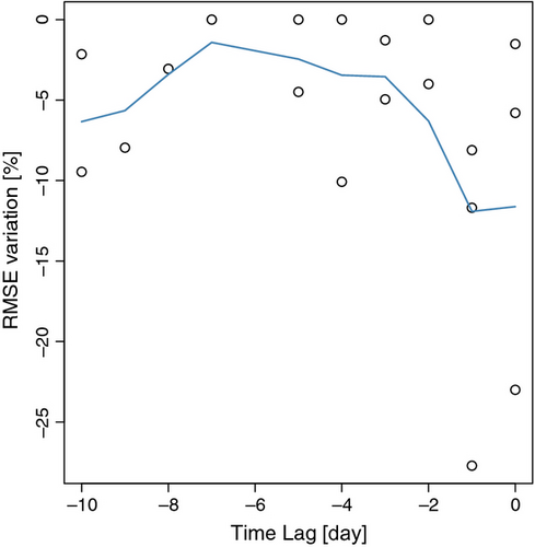
Finally, with the aim of detecting possible time-lags between respiration response and the peak of dGPP/dt, we ran the model with different time lagged dGPP/dt time series, starting from the dGPP/dt estimated on the same day up to a maximum lag time of 10 days after the measured RECO. The springtime peak of the rate of RECO might precede the dGPP/dt peak because the production of new leaves requires an increase of metabolic activity (e.g., translocation of carbon stored in woody tissues) that might precede the start of the carbon uptake period and the increase of GPP.
Statistical analysis
Estimation of model parameters and evaluation of model performance
Model parameters were estimated using the Levenberg–Marquardt method, implemented using the optim routine in R (version 2.14.0). Model parameter standard errors were estimated based on 500 bootstrap samples. As described by Efron & Tibshirani (1993), the obtained distribution of parameter estimates approximates the distribution of the ‘true’ model parameters.
Model performance was evaluated using a range of metrics (root mean square error, RMSE; coefficient of determination, R2; and mean absolute error, MAE; Janssen & Heuberger, 1995) to examine whether the inclusion of physiological phenology improved the description of the temporal variability of RECO. Modeling efficiency (EF), a measure of the coincidence between observed and modeled data, was also computed. EF ranges between -∞ to 1. A value of 1 corresponds to a perfect match between model and observation, while EF <0 indicate that the mean of the observations is a better predictor than the model. EF is sensitive to systematic deviation between model and observation (Janssen & Heuberger, 1995). Model statistics and residuals (observation-modeled value) were computed for the whole year and for each season (MAM, March–April–May; JJA, June–July–August; SON, September–October–November; and DJF, December–January–February) in order to evaluate the improvement in the description of the seasonal cycle of RECO.
 (8)
(8) equals the estimated within-sample residual sum of squares divided by n, and p is the number of parameters in the model. The model with the lowest AIC was considered the best model. The differences between the AIC (ΔAIC) computed for the TPdGPP (AICTPdGPP) model and the TPLinGPP (AICTPLinGPP) were computed. Negative differences indicated that the TPdGPP model, despite the higher complexity, was the best model formulation for the target dataset.
Spectral analysis of model residuals
Singular spectral analysis (SSA, Golyandina et al., 2001) was used to analyze periodicities in the residuals of TPLinGPP and TPdGPP, and to verify whether the seasonal bias in RECO decreased by including GPP development rate as an additional driver. The analysis was conducted both for the driver-observation set GPP-dGPP-RECO and NEEm-dfAPAR-NEEn.
- Because only days with <15% of gap-filled half-hours were retained, the time series of daily GPP and RECO contain gaps. We filled the gaps in the time series with an inherent SSA gap-filling strategy (Kondrashov & Ghil, 2006), as spectral analyses generally require gap-free records, whenever the FLUXNET methodology did not provide accurate estimates.
- The annual and monthly subsignals were extracted at each site from the observed RECO and the simulated series resulted from different model structures (TPLinGPP, TPdGPP).
- We retained only the original points (i.e., days not gap-filled during the step 1) from decomposed time series and computed the model-observation residuals of the different components of the time series (i.e., annual-seasonal, monthly).
- The variance of residuals from each component was computed for each time scale. The time-explicit decomposition allows for localizing mismatches between observations and models in frequency class and in time. This is a substantial advantage compared to conventional spectral analyses.
The annual-seasonal bins are defined here by periods in the interval (330:400) days (hereafter referred to as annual time scale), while the monthly component is defined by periods in the interval (30:60) days (hereafter referred to as monthly time scale).
Results
Evaluation of models performance
Across sites, the mean EF obtained for the two models, using the driver-observations GPP-dGPP-RECO, was 0.72 [interquartile distance 0.64–0.82] for the TPLinGPP model, and 0.76 [0.68–0.83] for the TPdGPP model (Table 3). For the driver-observations NEEm-dfAPAR-NEEn, the mean EF decreased to 0.66 (0.70) for the TPLinGPP (TPdGPP) (Table 4). By using the explicit description of physiological phenology, a decrease in RMSE of ~8% was achieved for GPP-dGPP-RECO and ~3% for NEEm-dfAPAR-NEEn. The largest improvement of model performance was observed at DE-Hai, FR-Fon, US-Bn2, IT-LMa, IT-Ro2, and US-MOz. Almost no improvement in model performance was observed at CA-Oas, FR-Hes, US-UMB, and US-LPH. The mean ΔAIC of −91.11 (−31.14) obtained for the driver-observations GPP-dGPP-RECO (NEEm-dfAPAR-NEEn) indicated that, even accounting for the higher models complexity (i.e., 1 parameter more), the TPdGPP model outperforms the TPLinGPP (Tables 3 and 4).
| Site | TPdGPP | TPLinGPP | ΔAIC | n | ||
|---|---|---|---|---|---|---|
| RMSE (gC m−2 day−1) | EF | RMSE (gC m−2 day−1) | EF | |||
| CA-Oas | 0.65 | 0.92 | 0.65 | 0.92 | 2.0 | 2914 |
| DE-Hai | 0.60 | 0.84 | 0.83 | 0.70 | −525.9 | 1873 |
| FR-Fon | 0.78 | 0.82 | 1.00 | 0.71 | −132.6 | 593 |
| FR-Hes | 1.49 | 0.63 | 1.49 | 0.63 | 2.0 | 3132 |
| IT-LMa | 0.67 | 0.73 | 0.74 | 0.67 | −41.8 | 507 |
| IT-Non | 0.81 | 0.80 | 0.81 | 0.80 | 2.0 | 794 |
| IT-PT1 | 0.77 | 0.83 | 0.78 | 0.82 | 2.0 | 802 |
| IT-Ro1 | 0.95 | 0.61 | 1.01 | 0.56 | −81.5 | 1895 |
| IT-Ro2 | 0.68 | 0.68 | 0.77 | 0.58 | −525.9 | 1170 |
| UK-Ham | 1.16 | 0.68 | 1.29 | 0.60 | −50.04 | 564 |
| US-Bar | 0.85 | 0.67 | 0.89 | 0.64 | −16.61 | 466 |
| US-Bn2 | 0.34 | 0.90 | 0.37 | 0.89 | −61.7 | 212 |
| US-Ha1 | 0.91 | 0.74 | 0.98 | 0.71 | −19.1 | 2358 |
| US-LPH | 1.29 | 0.53 | 1.30 | 0.53 | −25.4 | 440 |
| US-MMS | 0.65 | 0.83 | 0.66 | 0.83 | −56.2 | 2064 |
| US-MOz | 0.81 | 0.86 | 0.88 | 0.83 | −5.0 | 808 |
| US-Oho | 0.91 | 0.71 | 0.93 | 0.70 | −17.5 | 373 |
| US-UMB | 0.65 | 0.90 | 0.69 | 0.89 | −166.2 | 1537 |
| US-WCr | 1.68 | 0.78 | 1.75 | 0.76 | −13.6 | 1784 |
| Mean | 0.87 | 0.76 | 0.96 | 0.72 | −91.11 | |
| (0.25–0.75) | (0.65–0.95) | (0.68–0.83) | (0.76–1.08) | (0.64–0.82) | (−71.6–9.3) | |
| Site | TPdGPP | TPLinGPP | ΔAIC | n | ||
|---|---|---|---|---|---|---|
| RMSE (gC m−2 day−1) | EF | RMSE (gC m−2 day−1) | EF | |||
| CA-Oas | 0.73 | 0.90 | 0.74 | 0.90 | −32.44 | 2914 |
| DE-Hai | 0.74 | 0.76 | 0.88 | 0.66 | −279.89 | 1873 |
| FR-Fon | 1.19 | 0.58 | 1.20 | 0.57 | −2.31 | 593 |
| FR-Hes | 1.72 | 0.51 | 1.72 | 0.51 | 2.00 | 3132 |
| IT-LMa | 0.84 | 0.58 | 0.85 | 0.57 | −3.21 | 507 |
| IT-Non | 1.10 | 0.63 | 1.12 | 0.62 | −10.43 | 794 |
| IT-PT1 | 0.8 | 0.81 | 0.80 | 0.81 | 2.00 | 802 |
| IT-Ro1 | 1.06 | 0.52 | 1.16 | 0.42 | −146.39 | 1895 |
| IT-Ro2 | 0.68 | 0.68 | 0.77 | 0.58 | −3.21 | 1170 |
| UK-Ham | 1.16 | 0.68 | 1.29 | 0.60 | −50.04 | 564 |
| US-Bar | 0.85 | 0.67 | 0.89 | 0.64 | −16.61 | 466 |
| US-Bn2 | 0.36 | 0.89 | 0.46 | 0.82 | −43.14 | 212 |
| US-Ha1 | 1.04 | 0.67 | 1.03 | 0.67 | 21.79 | 2358 |
| US-LPH | 1.28 | 0.54 | 1.28 | 0.54 | 2.00 | 440 |
| US-MMS | 0.70 | 0.80 | 0.70 | 0.80 | 2.00 | 2064 |
| US-MOz | 1.00 | 0.78 | 1.01 | 0.78 | −4.98 | 808 |
| US-Oho | 1.06 | 0.61 | 1.12 | 0.56 | −15.84 | 373 |
| US-UMB | 0.78 | 0.86 | 0.79 | 0.86 | −15.01 | 1537 |
| US-WCr | 2.10 | 0.66 | 2.10 | 0.66 | 2.00 | 1784 |
| Mean | 1.04 | 0.70 | 1.07 | 0.66 | −31.14 | |
| (0.25–0.75) | (0.36–2.1) | (0.51–0.89) | (0.46–2.1) | (0.42–0.86) | (−24.53–2.0) | |
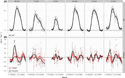
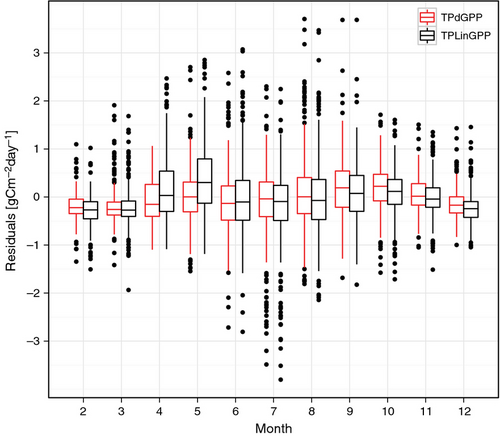
The use of the TPdGPP model led to a reduction of the model-observation mismatch, particularly in spring (Figs 2, 3, Table 5). The reduction of annual model residuals was not as relevant as that at seasonal time scale, likely because the seasonal bias in spring was partly compensated by negative biases in summer.
| Period | GPP-dGPP-RECO | NEEm-dfAPAR-NEEn | ||
|---|---|---|---|---|
| TPdGPP | TPLinGPP | TPdGPP | TPLinGPP | |
| DJF | −0.08 (0.80) | −0.11 (0.79) | −0.05 (0.80) | −0.09 (0.79) |
| MAM | −3.91 (0.90) | 7.82 (0.87) | 0.39 (0.84) | 0.44 (0.79) |
| JJA | −2.99 (0.87) | −7.19 (0.87) | 0.82 (0.80) | 0.83 (0.79) |
| SON | 0.17 (0.83) | 0.10 (0.82) | 0.29 (0.79) | 0.27 (0.80) |
| Year | 2.12 (0.91) | 4.31 (0.90) | 0.41 (0.86) | 0.42 (0.84) |
Spectral analysis of model residuals
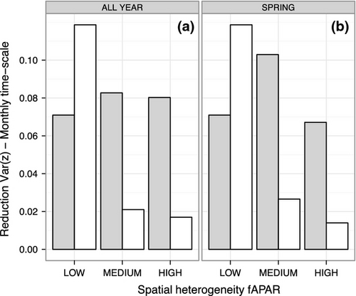
The boxplots of the model residual variance computed at each site for the monthly and annual time scales indicated a tendency toward lower variance on the monthly time scale for the TPdGPP model compared to the TPLinGPP model, for both driver-observation combinations (Fig. 4). On the annual time scale, a reduction in residual variance was also observed, however, differences were less pronounced than at the monthly time scale. For the driver-observations NEEm-dfAPAR-NEEn, the reduction of the residual variance at the monthly time scale was lower at sites with high spatial heterogeneity (Fig. 5). The latter was derived using the spatial standard deviation of JRC fAPAR computed in spring (Fig. 5a) and during the whole year (Fig. 5b).

Sources of uncertainty for the TPdGPP model
Comparing R2 values for the TPdGPP model driven by TS and TA indicates that the model driven by TA outperformed the model driven by TS in winter and early spring, while the R2 are similar in August and September (Fig. 6). The relative differences in RMSE between the TPLinGPP and TPdGPP model driven by TS and TA were generally low, except in a few sites (CA-Oas, IT-PT1, US-LPH, US-MMS, US-UMB; Table 6). At these sites we observed a small improvement of the performance using the TPdGPP model driven by TA, whereas, when using TS, the reduction of RMSE was larger, indicating that TS is likely the most important driver over these sites. The analysis conducted with a lagged response between dGPP/dt and RECO did not show a clear relationship between improvement in model performance and the time lag. Only the two sites with the largest improvement in model performances (i.e., DE-Hai and FR-Fon) were characterized by no or short lags between the physiological phenology and RECO, whereas at sites with a larger lag time, the improvement in model performance from introducing TPdGPP was less important (Fig. 7).
| Site | ΔRMSE(TA) (gC m−2 day−1) | ΔRMSE(TS) (gC m−2 day−1) |
|---|---|---|
| CA-Oas | 0.21 | 8.92 |
| DE-Hai | 27.42 | 30.30 |
| FR-Fon | 21.21 | 25.37 |
| FR-Hes | 2.39E-04 | 0.12 |
| IT-LMa | 9.38 | 12.03 |
| IT-Non | 0.26 | 5.81E-04 |
| IT-PT1 | 0.76 | 5.58 |
| IT-Ro1 | 6.16 | 6.61 |
| IT-Ro2 | 14.30 | 14.85 |
| US-Bar | 5.57 | 9.05 |
| US-Bn2 | 5.64 | 7.66 |
| US-Ha1 | 3.94 | 3.26 |
| US-LPH | 0.19 | 1.17 |
| US-MMS | 0.73 | 5.18 |
| US-MOz | 6.40 | 6.64 |
| US-Oho | 2.01 | 1.80 |
| US-UMB | 0.96 | 7.12 |
| US-WCr | 4.35 | 6.51 |
Discussion
Physiological phenology controls on ecosystem respiration
In a previous study, (Migliavacca et al., 2011) we showed that taking into consideration the dependency of RECO on some measure of short-term productivity (e.g., via coupling the base respiration to GPP) improved the skill of empirical RECO models significantly. Here, we show that, for a sample of deciduous broadleaved forests, RECO is controlled by climate (temperature and precipitation pulses) and canopy photosynthesis, and also by springtime physiological phenology. The latter can be approximated by the first derivative of daily smoothed GPP or fAPAR. The results obtained with the combination GPP-dGPP-RECO were more robust than those obtained with NEEm-dfAPAR-NEEn. This might be due to the higher noise in NEE time series, to scale mismatch between the eddy covariance flux tower and satellite footprint (Jung et al., 2008), and to the fact that nighttime NEEn reflects primarily the dynamics of soil respiration and, to a lesser extent, the dynamics of the aboveground respiration that are an important cause for the bias observed during the springtime period. Fig. 5 highlights that the largest reduction of the model-observation bias was observed in spatially homogeneous sites, suggesting that the proposed approach is sensitive to landscape heterogeneity. GPP is a more direct descriptor of the canopy photosynthetic capacity than fAPAR, which tracks the development of leaf area index. Interestingly, regardless of the driver-observations used (i.e., NEEm-dfAPAR-NEEn and GPP-dGPP-RECO), we identified a clear effect of physiological phenology on RECO. This finding leads to the proposed data-oriented semiempirical model that takes these linkages into account to improve the description of the seasonal cycle of RECO.
The analysis of the ratio of the R2 between TPdGPP models driven by TS and TA confirms the importance of air temperature during springtime (Fig. 6), suggesting that aboveground respiration plays an important role in spring. This supports the need to include physiological phenology as an additional driver in modeling RECO (Irvine et al., 2008). The seasonal dynamics observed in Fig. 6 are consistent with Davidson et al. (2006) and Giasson et al. (2013), who reported a spring pulse of aboveground respiration, leading to a minimum in the ratio between soil respiration and RECO in March and early April.
Limitations and future perspectives
Model performance statistics (Tables 3 and 4) show that the use of the explicit description of physiological phenology for some sites does not reduce the springtime bias in RECO. While all investigated sites are classified as deciduous broadleaved forests, some are composed of multiple tree species. Different species could have different and asynchronous phenological patterns that might confound the influence of physiological phenology on RECO at the ecosystem level. Moreover, considering that the RECO is observed at the ecosystem level with a variable footprint, the spatial heterogeneity of the canopy (Cescatti et al., 2012) might contribute to the poor model performances at some sites. For sites characterized by no or short lags between the physiological phenology and RECO, TPdGPP showed the largest improvement, whereas for sites characterized by larger lags the improvement of model performance by introducing TPdGPP was less (Fig. 7). For some sites, the springtime peak of RECO might precede the peak of dGPP/dt because production of new leaves requires an increase in metabolic activity (e.g., translocation of carbon stored in woody tissues) that would precede the onset of photosynthetic activity. This lag between foliage expansion and the development of photosynthetic capacity has been reported in the literature (e.g., Morecroft et al., 2003) and might be one of the causes of the limited improvement in model performance for some sites.
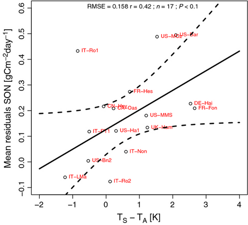
Future work is necessary to reduce the autumn bias of RECO, though less pronounced than the bias in spring, observed with the empirical model proposed by Migliavacca et al. (2011). The autumn bias might be related to the rapid decomposition of fresh litter inputs (DeForest et al., 2009), which is not accounted for by the empirical model. Decomposition in autumn may also be higher because of a large pulse of fine root turnover in addition to leaf litter fall. The inclusion of leaf or fine root litter pools would effectively turn our simple, empirical model into a more complex process-based model. Autumn bias might also be related to the difference between soil and air temperature, as soil temperature is higher than air temperature in the autumn. Thus, the TPLinGPP model driven by TA may lead to an underestimation of autumn respiration. In Fig. 8, the mean residuals during autumn at each site are correlated (r = 0.42 P < 0.1) with the mean difference between daily mean autumn TS and TA. In general, sites with higher model residuals in autumn are the ones with a more positive soil–air temperature difference (i.e., soil warmer than air).
Implication for data-oriented modeling
DeForest et al. (2006) showed that phenophase-specific models of soil respiration improve estimates of annual respiration. In fact, incorporating phenology into soil respiration models indirectly accounts for changes in environmental and/or biological factors that were not explicitly defined in the proposed model. The authors suggested that, ideally, the component fluxes of respiration should be modeled independently, or at least grouped according to time windows and environmental conditions during which common regulatory mechanisms (e.g., phenology) can be assumed. In this study, we proposed an empirical model for RECO that includes the first derivative of GPP (or fAPAR) to explicitly account for the physiological phenology-related pulse of RECO during spring (from bud-break to leaf unfolding), before reaching the maximum LAI.
Our results suggest that the proposed model structure reduces the spring-summer bias in RECO estimates. Annual estimates of RECO are also less biased even though to a lesser extent than at seasonal time scale. This is probably due to the compensation of the model bias in spring (positive) and summer (negative) without the explicit dependency of RECO on physiological phenology. The spring bias is particularly relevant to global carbon cycle studies for several reasons. First, spring is considered the most critical period determining the interannual variability of the net ecosystem CO2 uptake (Le Maire et al., 2010) in ecosystems that are not characterized by summer drought and, therefore, an accurate modeling of respiration will likely improve estimates of the net CO2 uptake in this crucial period. Second, the mean springtime and annual bias introduced by using the two different modeling approaches at global scale results in a difference in the net carbon uptake of about 1.4 PgC yr−1 at the annual time scale, while a difference of 0.6 PgC and 0.8 PgC are expected in spring and summer, respectively. These results were obtained by multiplying the average residuals by the global coverage of deciduous forests in m2 [1752105 km2 according to Hansen et al. (2000)]. The springtime bias in RECO might significantly affect the estimates of land–atmosphere CO2 fluxes obtained from atmospheric inversion models when these data are used as priors. This is particularly relevant for regional-scale inversions because the distribution of temperate deciduous forests is divided mainly between Northern Eurasia and Northeastern America.
In conclusion, our study suggests that it is necessary to account for the dependence of ecosystem respiration on short-term productivity (e.g., daily GPP) and on the physiological phenology to guarantee reliable simulations of RECO of deciduous broadleaved forests. By explicitly including the effects of physiological phenology on RECO, we found that spring and summertime biases observed in previous studies are significantly reduced. This implies that for global or regional-scale application of data-oriented empirical models, some measure of rate of development of physiological phenology needs to be included to improve the simulation of seasonal and interannual variability of RECO. This improvement is necessary to strengthen the analysis and interpretation of the seasonal cycle of the global CO2 growth rate and annual carbon balance. Although the present study using the FLUXNET database clearly reveals a tight linkage between physiological phenology and ecosystem respiration in deciduous forests, future experimental efforts should focus on refining the mechanistic understanding of this linkage. From a modeling perspective, future work is also needed to improve the simulation of the respiration pulse in autumn.
Acknowledgments
This work used eddy covariance data acquired by the FLUXNET community and in particular by the following networks: AmeriFlux (U.S. Department of Energy, Biological, and Environmental Research, Terrestrial Carbon Program (DE-FG02-04ER63917 and DE-FG02-04ER63911)), AfriFlux, AsiaFlux, CarboAfrica, CarboEuropeIP, CarboItaly, CarboMont, ChinaFlux, Fluxnet-Canada (supported by CFCAS, NSERC, BIOCAP, Environment Canada, and NRCan), GreenGrass, KoFlux, LBA, NECC, OzFlux, TCOS-Siberia, and the USCCC. We acknowledge the financial support to the eddy covariance data harmonization provided by CarboEuropeIP, FAO-GTOS-TCO, iLEAPS, Max Planck Institute for Biogeochemistry, National Science Foundation, University of Tuscia, Université Laval, Environment Canada and US Department of Energy and the database development and technical support from Berkeley Water Center, Lawrence Berkeley National Laboratory, Microsoft Research eScience, Oak Ridge National Laboratory, University of California – Berkeley and the University of Virginia, and the IceMe of NUIST. The authors would like to thank all the PIs of eddy covariance sites, technicians, postdoctoral fellows, research associates, and site collaborators involved in FLUXNET who are not included as coauthors of this paper, without whose work this analysis would not have been possible. ADR acknowledges support from the National Science Foundation, grants DEB-1114804 and EF-1065029. The authors thank Morgan Furze for editing the article for style and grammar, and the anonymous reviewers and the editor for the comments that improved the readability of the article.


