A high-resolution approach to estimating ecosystem respiration at continental scales using operational satellite data

Model development

Ecosystem respiration consists of Autotrophic Respiration (Ra), which is the growth and maintenance respiration of leaves, stems, and roots, and Heterotrophic Respiration (Rh), which accounts for belowground decomposition by the microbes and soil fauna (e.g., Raich & Tufekciogul, 2000; Ryan & Law, 2005),

(1)

NEE is defined as the difference between Re and GPP:

(2)

It is not feasible to disentangle the complex interactions of surface and subsurface processes contributing to Re by means of remote sensing. Yet, on the time-scale of days, simplified empirical approaches have proven instrumental to estimating Re in its seasonality and magnitude (Richardson et al., 2006a; Reichstein & Beer, 2008; Migliavacca et al., 2011). Our modeling strategy is based on the following assumptions. Temperature (Lloyd & Taylor, 1994; Raich & Tufekciogul, 2000) and plant productivity (Janssens et al., 2001; Kuzyakov & Gavrichkova, 2010) are the predominant drivers of short-term temporal variation, which can be limited by water stress (Raich & Schlesinger, 1992; Reichstein et al., 2007). We link variation in magnitude of Re between sites and years (interyear differences, e.g., due to disturbances and management) to mean annual plant productivity (Janssens et al., 2001; Yuan et al., 2011) and to mean annual temperature (Raich & Schlesinger, 1992; Bond-Lamberty & Thomson, 2010). Furthermore, we assume that plant productivity can explain short-term variations in Re as well as long-term and spatial differences, because GPP is directly linked to Ra and because organic matter sustains above- and belowground decomposition through litter fall (e.g., Bahn et al., 2010). We link each of these semi-empirical dependencies to operational remote sensing products below.

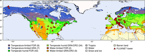
Parameters are estimated for six aggregated functional biomes, which are based on Koeppen-Geiger climate classification (Peel et al., 2007; ORNL, 2010) and the International Geosphere-Biosphere Program (IGBP) classification scheme from the MODIS land cover product (Friedl et al., 2002). We stratify climate classes based on their temperature and precipitation regime into three climate types: (i) Temperature-Limited (TL, cold and polar climates), (ii) Temperate and Humid (TH, temperate, not summer dry) and (iii) Water-Limited (WL, semiarid with summer dry period). Further, we divide each climate type into two functional aggregated land cover types: (i) forests (FOR) and (ii) non-forested natural vegetation or croplands (GRA/CRO). Only vegetated areas are investigated. Figure 1 displays the global distribution of aggregated biomes.

To account for spatial and seasonal variability separately, we partition Re observations into the site-specific reference respiration rate (Re_ref) and the remaining standardized respiration rate (Re_std), which is the seasonal variation, detrended for site characteristics and thus predictor responses are smoothed across sites (Fig. 2).

Reference Respiration Rate (Re_ref). Re_ref is the respiration rate at the temperature T_ref (°C), which describes differences in magnitude between sites and years. T_ref is set to the approximate mean springtime temperature (Day of Year 96-144) for each climate type: T_{ref_TL} = 0 °C, T_{ref_TH} = 12 °C and T_{ref_WL} = 13 °C. We find that Re_ref becomes less suitable to capture site characteristics at higher T_ref values. Particularly among WL, sites water-stress confounds the temperature signal above 13 °C. Re_ref is extrapolated at T_ref through a polynomial surface from the reference data for each site and year.

In RECO, Re_ref is estimated as follows:

(4)

where EVI_mean is mean annual springtime EVI (observations within T_ref ± 3 °C, as nighttime LST equivalent, and from first half-year), LST_mean is mean annual daytime LST (LST_d) and p_1-3 are free parameters. For climate types TL and WL, Re_ref parameterization is not further split into land cover classes FOR and GRA/CRO, because data availability is limiting. Figure 3 displays Re_ref dependencies to EVI_mean and LST_mean.

Standardized Respiration Rate (Re_std). Re_std is the ratio of Re and Re_ref. For all fitted biomes that are not water-limited (TL-FOR, TL-GRA/CRO, TH-FOR and TH-GRA/CRO), Re_std is estimated as follows:

(5)

where LST_n is nighttime LST (°C) and EVI refers to standardized EVI (8-day EVI divided by EVI_mean) and p_4-8 are free parameters. We estimate Re_std in case of snow cover from a separate LST_n only fit (Fig. 4).

Water stress shows a considerable impact at WL sites, which we directly account for through the difference between daytime and nighttime LST (LST_dif) (Cai et al., 2007). This approach exploits radiation properties of changing surface soil moisture content (Schmugge, 1978; Verstraeten et al., 2006; Wang & Qu, 2009). Further, we also account for water stress indirectly through EVI (e.g., Gu et al., 2007; Schnur et al., 2010). During periods of water limitation the temperature dependence of Re_std is no longer valid. Therefore, we calculate Re_std for the WL biome during the dry period as follows:

(6)

The remaining season in WL climates is estimated as follows:

(7)

We define the dry season to occur between Day of Year (DoY) 136 and 272 as an empirical finding in the data. These dates delimit the summer cutback of the mean seasonal course across WL data (Fig. S2).

Fluxnet data and parameter estimation

RECO parameter estimation is based on data from the Fluxnet program between 2000 and 2009 (ORNL, 2011). We employ air temperature (Ta) and Re, which is provided as a temperature interpolation from nighttime net carbon fluxes (Reichstein et al., 2005). We utilize gap-filled and quality-assessed 8-day average data (Level 4, well mixed conditions) (Papale & Valentini, 2003) and we filter data by quality flag (qc > 0.9). A threefold gliding window filter is applied to smooth Re observations. To account for footprint heterogeneity we only incorporate sites which are situated within four pixels of the same 500 m aggregated MODIS land cover type (FOR or GRA/CRO). Overall, 100 sites meet our demands of data quality and footprint homogeneity and are distributed between 28.61° and 71.32°N and between −157.41° and 35.05°E (Fig. 1). Although sites are not equally distributed across biomes, and only situated in the northern hemisphere, most major non-tropical biomes are represented.

Parameters are estimated by nonlinearly minimizing the sum of squared residuals, weighted by its uncertainty (Lasslop et al., 2008). LST_n and EVI show generally high level of multicollinearity; we allow values up to 0.8. A fivefold cross-validation procedure is employed to estimate and validate the parameter set. For each cycle, 80 percent of the available sites are used for model calibration and 20 percent are detained for validation. Each site is used for validation exactly once, and parameters are never evaluated against calibration sites. Continental-scale RECO application is based on parameters retrieved from the entire site data to assure most robust parameters (Table S3, S4).

The following evaluation criteria are employed: (i) correlation coefficients (r) calculated using the Pearson method, (ii) Coefficient of determination (R²), (iii) root mean square error (RMSE), (iv) mean biased error, MBE = sum(observed-predicted)/n, (v) Estimation Uncertainty (OEU), the mean absolute error divided by mean prediction, and (vi) Akaike's Information Criterion (AIC), which is used for equation performance comparison.

MODIS data

MODIS LST is retrieved from seven Thermal Infrared (TIR) bands (Wan & Dozier, 1996). We employ the 1 km MOD11A2 and MYD11A2 V5 LST products, which are 8-day average values of cloud free observations featuring day- and nighttime estimates, respectively. We omit observations if the qc flag indicates ‘bad raw data quality’ or if ‘average LST error’ > 1 K (Wan & Li, 2008; Coll et al., 2009).

We use the atmospherically corrected MOD09A1 V5 8-day surface reflectance (best observation in 8 days) at 500 m resolution to calculate EVI as follows:

(8)

where G is a gain factor, ρ is surface reflectance at the Near Infrared (NIR), red and blue band, L is the canopy background adjustment, and C1, C2 are coefficients of the aerosol resistance term. We adopt coefficient values from the MODIS EVI algorithm, L = 1, C1 = 6, C2 = 7.5, and G = 2.5. EVI over snow is ill-defined; therefore, we mask EVI if Normalized Difference Snow Index (NDSI) exceeds −0.1 (Salomonson & Appel, 2004). NDSI is calculated as follows:

(9)

where ρ is the reflectance in the green and in the Short Wave Infrared band.

Land cover is assessed using the yearly IGBP MCD12Q1 V5 500 m product. Data from 2001 to 2005 are available to this study, filtered with the quality assessment flag (confidence > 50%) and averaged across years to one static map. In situ land cover information is not considered, because it does not necessarily account for the entire pixel footprint.

All 8-day MODIS products are averaged over pixels indicating the same aggregated land cover class within a 3 × 3 km subset. Primarily, we use Terra products, but we also use Aqua data for gap-filling, which we linearly adjust to account for an offset due to different overpass times (Crosson et al., 2012) (Fig. S2).

DGVM for comparison

We use process-based Re simulations from LPJmL as an independent source to compare large-scale spatial Re patterns. The purpose of the comparison is to gain bidirectional confidence in both approaches for regions where they agree and also to identify regions of uncertainty. The LPJmL ecohydrological modeling framework simulates global vegetation and carbon dynamics at 0.5° resolution (Sitch et al., 2003). We force LPJmL with the monthly climatology of the Climate Research Unit's (CRU) TS 3.1 (1901–2009) for temperature, cloudiness and wet days (Mitchell & Jones, 2005) and by the Global Precipitation Climatology Centre's (GPCC) precipitation data (Version 5) (Rudolf et al., 2010). Transient runs follow a 5000-year spinup recycling the first 30 years of input climatology and, in addition, a 390-year agriculture spinup with prescribed historical land use distribution (Fader et al., 2010).

Carbon fluxes (gross primary production, auto- and heterotrophic respiration) and pools (leaves, sapwood, heartwood, storage organs, roots, litter and soil) are mechanistically represented, in direct coupling with the water balance (Gerten et al., 2004) and vegetation dynamics for natural (9 plant functional types, PFT) as well as for agricultural land cover (12 irrigated and rain-fed crop functional types, CFT, and pastures) (Bondeau et al., 2007). Permafrost dynamics along with an updated water-balance implementation are described in Schaphoff et al. (2013).

Ra is calculated from the difference of GPP and NPP. Maintenance respiration is calculated individually for each tissue type (leaf, sapwood, and root), based on carbon–nitrogen ratios, air and soil temperature, tissue biomass, and phenology. The temperature sensitivity of Ra follows a modified Arrhenius equation (Lloyd & Taylor, 1994), which describes a decreasing temperature sensitivity with increasing temperature, but parameterization remains constant across biomes and PFTs. Furthermore, 25% of the remainder from GPP and maintenance respiration is substracted as growth respiration, the remainder is NPP. Rh is the sum over carbon emissions from three carbon pools (litter, intermediate, and slow soil organic matter), for each PFT. Each pool has an assigned turnover rate (0.3, 0.03, and 0.001 a⁻¹ at 10 °C, respectively) and decomposition rates are calculated as a function of turnover rate, air and soil temperature, and moisture. The temperature sensitivity of Rh equals the Lloyd & Taylor (1994) dependency. Because RECO and LPJmL employ inherently different approaches to calculate Re, we cannot compare single parameters individually, but only temperature sensitivities and Re estimations itself.

RECO parameterization

In order to aggregate functional biomes, we find that it is inevitable to distinguish three major climate classes TL, TH, and WL, to separate temperature- and water-limited sites. Further, it appears important but less essential to distinguish land cover classes, because responses are not substantially different across land covers. Nevertheless, we can further divide significantly forested and non-forested land cover classes within each climate type. Parameters become insignificant if to further separate agricultural land, due to insufficient amount of data, but driver responses between CRO are GRA are not critically different (Fig. 4). Overall, incorporated Fluxnet data allow to parameterize RECO for six aggregated biomes significantly. Parameter sets for Re_ref and Re_std and each fitted biome are presented in Tables S3 and S4 in the supplementary information.

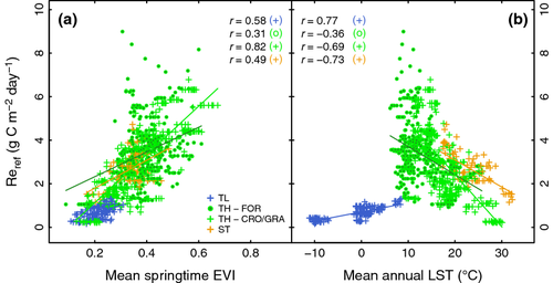
Re_ref shows robust responses to EVI_mean and LST_mean, which can be approximated linearly (Fig. 3). EVI_mean has positive slopes with steepest increase among GRA/CRO sites. Temperature limitation among TL sites is characterized by a positive Re_ref response to LST_mean, while all other sites follow a negative slope. Variation among TH-FOR sites, however, is explained to a lower degree compared to other biomes, which adds substantial uncertainty to the overall RECO performance.

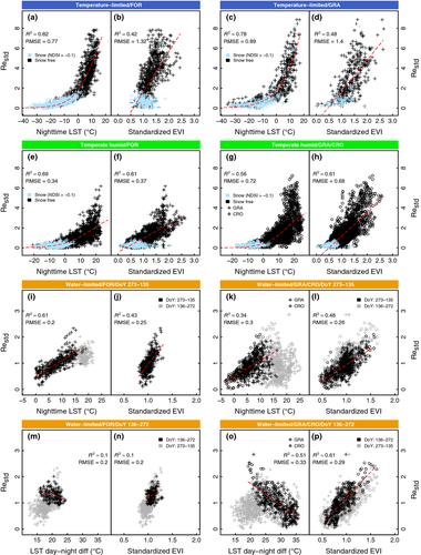
Figure 4 illustrates Re_std driver responses. The ‘sigmoidal’ function (Fang & Moncrieff, 2001) exhibits overall best performance to approximate the LST_n response across biomes according to Akaike's Information Criterion (Burnham, 2004). It is flexible enough to match the declining temperature sensitivity that characterizes our data (Fig. 4, Fig. S3). Competing equations and their performance measures are listed in Table S5.

Water-limitation is characterized by a LST_n response that levels off and becomes ambiguous during that period of time. We find low (no) impact of water-limitation on TH (TL) sites, but strong impact on WL sites during the period DoY 136 to 272 (Fig. 4i, k). To account for water stress through LST_dif, it was necessary to stratify WL data into dry and non-dry season, because LST_dif is only significant during the time of water-limitation (Fig. 4m, o). Here, LST_dif explains a large amount of the variation in Re_std following a strong negative response (Fig. 4o). The LST_dif response at FOR sites is less pronounced compared to GRA/CRO sites (Fig. 4m), because trees are less sensitive to temporary drought impact compared to grass and shrubs, due to deeper rooting and higher water storage capacity (Pereira et al., 2007).

We find EVI is a strong predictor across all climate and land cover types and shows robust responses also outside of the growing season and during periods of water-limitation (Fig. 4). The EVI response appears unsaturated and can be approximated with a linear function. We do not find a time-lag between EVI and Re_std at the 8-day scale, which confirms Kuzyakov & Gavrichkova (2010).

MODIS LST correlates closely with Ta (r_LSTn = 0.97), while LST_n approximates Ta better than LST_d, which shows a systematic bias (slope_LSTn = 0.96, slope_LSTd = 0.72). LST_d is affected by light and shadow effects, which limits the ability to predict the baseline temperature (Sims et al., 2008; Wan, 2008). In turn, annual means of LST_d explain more variation in Re_ref across all biomes than means of nighttime LST, which can be associated with higher sensitivity of LST_d to surface conditions. Accordingly, we use LST_n as a driver for Re_std and mean LST_d for Re_ref. Mean EVI of all observations during one year explains less variation in Re_ref than mean EVI of springtime observations. The definition of ‘springtime’ is an empirical finding (T_ref ± 3 °C, from first half-year). Further, EVI divided by mean springtime EVI (which we call standardized EVI), explains more variation of Re_std across all biomes than plain EVI, because it detrends the EVI response for site-specific slopes. The Snow definition through NDSI > −0.1 (Eqn. 9) outperforms the MODIS snow index (Fig. S1). MODIS IGBP land cover agrees with in situ IGBP land cover at 50 of 100 sites, and at 76 of 100 sites for the aggregated classes (Table S2).

RECO evaluation

Final overall model accuracy for 8-day Re predictions based on fivefold cross-validation is R²_{Re_overall} = 0.616, RMSE_{Re_overall} = 1.321 [g C m⁻² d⁻¹]. Lowest accuracy is achieved for the mid-latitude TH biome and increases with temperature-limited and water-limited biomes (Fig. 5c, f, i). Overall estimation uncertainty accounts to ± 34.5 percent with little variation across biomes and the model regression slope and MBE do not indicate a substantial systematic bias [slope_overall = 0.91, MBE = 0.051 (g C m⁻² d⁻¹)].

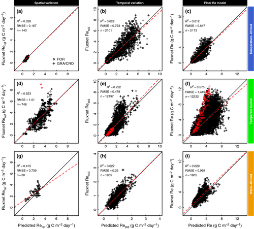
Temporal variability (Re_std) is generally explained to a higher degree compared to spatial variability (Re_ref) (Fig. 5) (R²_{Reref_overall} = 0.682, R²_{Restd_overall} = 0.778). Uncertainty in Re_ref has a direct leverage effect on final Re estimates (Fig. 5d-f), therefore particularly mid-latitude forest sites (TH-FOR) contribute considerably to overall Re uncertainty, which is a result of the poor TH-FOR response to EVI_mean and LST_mean (Fig. 3). However, differences in overall Re accuracy between land cover classes are not substantial, only TL-FOR stands out with exceptionally accurate estimates [R²_TL-FOR = 0.857, RMSE_TL-FOR = 0.593 (g C m⁻² d⁻¹)] (Table S6).

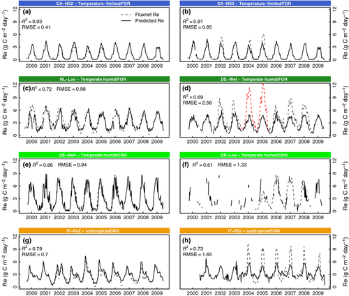
In Figure 6, we show for each biome type time-series for sites with good agreement (left column) face to face with sites revealing typical shortcomings (right column). In general, seasonal variation is tracked robustly across all climate and land cover classes. RECO also shows capacity to reproduce senescence-induced cutback during the dry season in water-limited climates (Fig. 6g) and exhibits reasonable sensitivity to interannual variability. The first of the negative examples (Fig. 6b) shows unusually low summer Fluxnet values in 2003, despite regular signals in EVI and LST and without being documented as disturbance event. Second, Fig. 6d (site DE-Wet, also highlighted in Fig. 5d–f) measures respiration rates well above the average TH forest site, which has been associated with specific micro-meteorological conditions in combination with inhomogeneous and sloped tower footprint (Rebmann et al., 2010). These two examples illustrate the impact of possible errors in the Fluxnet record on the model evaluation, but they also reveal that the model parameterization is robust against such outliers. Figure 6f highlights the problem with data availability from the MODIS sensor. The delivered quality flag rejects a substantial fraction of the 10-year time-series. It is mostly cloud cover that is an crucial issue for missing data, which has a considerable impact on the calculation of annual sums in some regions. As for Fig. 6h, the subtropical cropland site IT-BCi shows a unique pattern: Isolated respiration peaks remain crudely underestimated. Individual rain events after periods of drought have been attributed to increased soil carbon effluxes that can exceed rates under well-watered conditions and for which the temperature dependence temporally gets overridden, the so-called ‘Birch-effect’ (Xu & Baldocchi 2004, Reichstein & Beer, 2008). These short-term peak events are therefore not to be detected in the EVI and LST signal.

Spatial pattern comparison with LPJmL

Re annual sums for 2003 across North America and Europe, predicted by RECO and simulated by LPJmL, are illustrated in Fig. 7. Both methods estimate similarly characteristic large-scale spatial patterns. For example, the distinct west-east soil moisture gradient throughout North America with peak values at the south and south-east coastline, the US south-west desert regions and the North-American west coast and its patchy patterns around British Columbia are modeled similarly. Spatial patterns across Europe are also reasonably well in agreement, for example, high values in western France to low values along the European Alps and the elevated footprint of the Carpathians to the pronounced south-east border of the Black Sea and the greening of the Nile delta.

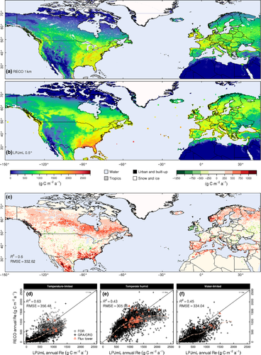
A difference map of LPJmL minus RECO annual sums at the 0.5° grid (Fig. 7c) reveals specific regions of uncertainty. The overall agreement between both models for all pixels is R² = 0.6, RMSE = 332.62 [g C m⁻² a⁻¹]. While mid-latitude regions between 40°N and 55°N are well in agreement, LPJmL simulates consistently higher values in boreal and high-latitude regions in Canada and north-eastern Europe, but also in subtropical regions in south-eastern US and Mexico and along the coastline of the Mediterranean Sea. One of the rare areas where RECO predicts substantially higher values than LPJmL is Ireland and south-western UK. Mean biased error (MBE) between RECO and LPJmL accounts to −174.4 [g C m⁻² a⁻¹], indicating a consistent over-prediction by LPJmL. Figure 7 d-f show scatter-plots of RECO versus LPJmL pixels for the above presented map, including Flux tower locations. The mean error is highest among TL and WL biomes and decreases where tower distribution is dense, that is, in the TH biome (despite higher annual sums). Importantly, regions where both models diverge most significantly are represented by Flux towers at least to some degree. Regions with no tower representation mostly have very low annual sums in TL and WL, where in turn both models are sufficiently in agreement. Given this, Fluxnet towers appear to form a valid reference tool and to be appropriate for up-scaling to the study region.

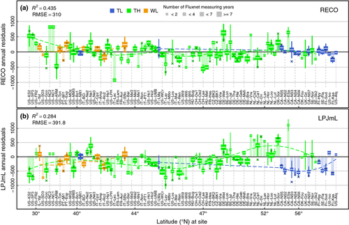
Taking Fluxnet sites for reference, LPJmL annual errors exceed those from RECO by one-quarter (RMSE_{LPJmL_annual} = 396.7 [g C m⁻² a⁻¹], and RMSE_{RECO_annual} = 305.8 [g C m⁻² a⁻¹], resp.). But most importantly, LPJmL shows systematic positive bias throughout all investigated biomes. MBE for annual sums accounts to MBE_LPJmL = −153 and MBE_RECO = 21.3 [g C m⁻² a⁻¹], respectively. Ordered by latitude, Fig. 8 marks mean annual residuals for each site. The LPJmL trend-line across latitudes remains with negative values (positive bias) for all but a few central European sites. Carbon efflux is simulated most excessively at the TL biome (CA-NS2/3, FI-Hyy, SE-Fla, FI-Sod, FI-Kaa) and sites among the south-east US (US-KS2, US-SP3, US-Goo). The trend of RECO annual residuals is located reasonably close to zero for all biomes, except for the south-east US, where RECO underestimates annual sums as much as LPJmL overestimates, which renders this as a region of specific uncertainty. Interestingly, IE-Dri and UK-Esa represent the region where RECO predicts higher values than LPJmL, but Fig. 8 indicates that this is due to underestimation in LPJmL.

Evaluation of mean monthly estimates is shown in Figure 9. While the monthly bias pattern is consistent with the bias of annual sums, mean monthly estimates show considerably higher accuracy in both models (Fig. 8, 9). RECO achieves smaller mean monthly errors compared to LPJmL (RMSE_RECO = 1.22 and RMSE_LPJmL =1.59 [g C m⁻² d⁻¹], resp.), which shows positive bias across all biomes, most pronounced for TL sites (slope_TL = 0.45, slope_TH = 0.72, slope_WL = 0.89). In comparison, RECO shows very small bias in all three fitted biomes (slope_TL = 0.97, slope_TH = 0.92, slope_WL = 1.03). The error between RECO and LPJmL at tower pixels is 1.42 [g C m⁻² d⁻¹], which indicates that LPJmL agrees better with RECO than with tower data. Interestingly, this value stays remarkably stable if all pixel are included (RMSE_{RECO-LPJmL-all} = 1.41 [g C m⁻² d⁻¹]).

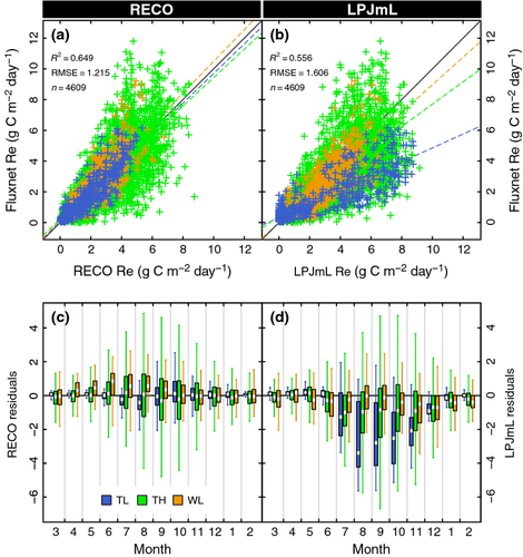
Evidently, residuals increase with increasing Re over the growing season in both models (Fig. 9c, d). RECO residuals indicate an underestimation during WL summer months, but no distinct seasonal pattern for the other biomes. LPJmL residuals show a considerable seasonal pattern with distinct negative median residuals during the growing season with TH and TL biomes. Median residuals in the TL biome exceed -2 [g C m⁻² d⁻¹] from June to September.

RECO evaluation

The RECO model demonstrates that Fluxnet Re observations can be estimated with an applicable degree of accuracy across major global biomes using only satellite remote sensing data. Its semi-empirical approach proves instrumental in capturing a high amount of spatio-temporal variability. The definition of Re_ref as the reference respiration rate factor is key to segregate temporal and spatial variations, which is crucial to designing an operational model, because site characteristics are associated with Re_ref and temporal variation is standardized across sites. Reichstein et al. (2007) and Migliavacca et al. (2011) present such an approach at the plot scale, and Yuan et al. (2011) provides a global map of Re_ref based on GPP estimates from a light use efficiency model. But to our knowledge, this concept has not been subject to an operational remote sensing-based study applicable to large scales at the 1 km resolution.

Incorporated drivers serve as higher level proxies for more complex underlying sub-processes. For example, at very high latitude sites, LST_n explains more variation in Re than in situ air temperature, which is remarkable, since LST is a space-borne product with a considerable bias against Ta measurements (RMSE = 2.84 °C). The LST product is specifically suitable for monitoring ecosystem conditions and stresses, in that it is not only a proxy for temperature but also for other processes such as vapor pressure deficit (VPD). For example, reduced stomatal conductance, that is, higher VPD, and reduced vegetation cover during periods of drought cause elevated daytime LST (Hashimoto et al., 2008; Sims et al., 2008), which hence characterizes ecosystem states more generally. Moreover, plant productivity is affected by water stress, and associated senescence effects cause reduction in vegetation canopy chlorophyll content, which can be observed by vegetation indices. This explains why EVI significantly contributes to tracking Re during periods of water stress. At the pixel-scale, EVI is also capable to accounting for disturbances and management to a certain degree. EVI contributes to Re_std estimates as a high-level proxy for plant productivity, plant physiognomy and plant water stress. Compared to previous remote sensing-based studies (Vourlitis et al., 2003; Gilmanov et al., 2005; Yamaji et al., 2007; Schubert et al., 2010), we directly account for plant water stress through LST_dif which extends the operational area to semiarid climates. Most existing approaches also exploit the temperature dependence of respiration during periods of water limitation, which we have shown to be ambiguous. Although all RECO predictor variables are selected empirically, we follow physiological dependencies, which marks RECO as a semi-empirical approach.

Overall, RECO accuracy is on a par other recent approaches: Kimball et al. (2009), for example, estimated Re for boreal and Arctic biomes with a remote sensing-based model accounting for soil moisture (AMSR-E data, currently out of order, as of September 13, 2013) and three different soil carbon pools. They achieve mean site-level accuracy of R² = 0.54 and RMSE = 0.73 [g C m⁻² d⁻¹]. For that biome, we calculate: R² = 0.82 and RMSE = 0.58 [g C m⁻² d⁻¹]. Further, overall RECO results are close to the in situ 8-day study by Migliavacca et al. (2011). They found an overall fit of R² = 0.72 and mean RMSE = 1.06 [g C m⁻² d⁻¹], while we calculate for a very similar data set, but based on remote sensing input: R² = 0.69 and mean RMSE = 1.24 [g C m⁻² d⁻¹]. While Migliavacca et al. achieve a higher degree of accuracy in annual sums, the additional uncertainty in our study might be due to the spatial mismatch between tower footprint and satellite pixel. Jung et al. (2011) calculate monthly values with performance measures of: R² = 0.69 and RMSE = 1.04 [g C m⁻² month⁻¹] which slightly exceed our values [R² = 0.65 and RMSE = 1.21 (g C m⁻² month⁻¹)].

We calculate Re_ref on a yearly basis to account for interannual variation, disturbances, and trends. Due to its multiplicative design (Eqn. 3), errors in Re_ref have a distinct leverage effect on final Re estimates. This is particularly the case among TH sites, where model residuals are mainly induced by considerable uncertainty associated with Re_ref. A temporally static Re_ref, however, leads to lower overall accuracy measures (not shown). In general, annual means of EVI and LST explain a sufficient amount of the variability in Re_ref across non-tropical biomes. Re_ref depends strongly on photosynthesis (e.g., Janssens et al., 2001; Yuan et al., 2011) and thus has often been modeled based on LAI observations (Hibbard et al., 2005; Lindroth et al., 2008; Migliavacca et al., 2011). But in our study, EVI and mean EVI consistently outperform LAI and mean LAI, respectively. We assume that mean EVI observations can roughly account for substrate availability and biomass and also to a low degree for labile soil carbon pools. However, we expect that more accurate information on slow soil carbon pools, substrate availability, and soil structure would considerable contribute to better explaining variations in Re_ref between sites and years. We investigated biomass products from in situ and remote sensing-based data (Blackard et al., 2008) and also soil carbon data (Global Soil Data Task, 2000), without finding a significant contribution (not shown). Current advances in remote sensing of terrestrial biomass (e.g., Bellassen et al., 2011; Saatchi et al., 2011) could contribute to reduce uncertainty. The goal of this study, however, was to develop a single-sensor operational product that fits into the existing MODIS product family in terms of spatio-temporal resolution, to allow the combination with existing GPP products.

A positive relation between Re_ref and mean LST is an indicator for temperature limitation (Fig. 3). The negative dependency between Re_ref and mean LST among sites that are not temperature-limited can be associated with two different reasons. First, the phenological state at temperature T_ref varies between sites (i.e., sites with lower mean annual temperature are more advanced into the growing season than warmer sites and thus baseline respiration is higher). Second, as it has been shown frequently, the apparent temperature sensitivity decreases with increasing mean temperature (see following paragraph). Mean LST is sensitive to elevation gradients and the climate classification only accounts for elevation at a large scale. Nevertheless, the response to Re_ref is reasonably strong.

The true temperature sensitivity of respiratory processes and the question if it varies systematically between ecosystems and over time is still under debate (Davidson & Janssens, 2006; Gu et al., 2008; Kirschbaum, 2010; Mahecha et al., 2010; Yvon-Durocher et al., 2012). The well-known exponential Q₁₀ function (Black et al., 1996) is characterized by a constant Q₁₀ over space and time, where Q₁₀ is the factor by which respiration multiplies in response to a 10° temperature increase. Lloyd & Taylor (1994) show that an exponential increase underestimates low and overestimates high respiration measurements and they present a modified Arrhenius type function with a declining Q₁₀ at higher temperatures. More flexible s-shaped functions were developed (Kirschbaum, 1995; Fang & Moncrieff, 2001; Del Grosso et al., 2005) to even better meet field measurements and it has been shown that the apparent temperature sensitivity varies spatially with higher sensitivities among colder climates and lowest values among deserts (e.g., Tjoelker et al., 2001; Zhou et al., 2009; Chen et al., 2010). Variations in Q₁₀ are generally attributed to temperature acclimation during the season and limitations by water and biomass, as substrate availability decreases with increasing temperature (Ryan, 1991; Raich & Schlesinger, 1992). On the contrary, Yvon-Durocher et al. (2012) were recently able to show that the short-term temperature sensitivity between different ecosystems is very similar and Schindlbacher et al. (2009) concludes that root autotrophic and soil heterotrophic respiration responded equally to temperature. Moreover, Reichstein & Beer (2008) attributed the Q₁₀ decline at higher temperatures to interactions with soil moisture limitations, while Mahecha et al. (2010) circumvented those confounding effects and concluded with a spatio-temporally static Q₁₀ of 1.4. However, despite the discussion on the true temperature sensitivity, at the ecosystem level the Lloyd & Taylor function remains one of the most common temperature sensitivities in recent empirical and process-based models (e.g., Sitch et al., 2003; Reichstein et al., 2007; Schubert et al., 2010; Migliavacca et al., 2011).

In our study, we examine large-scale ecosystem-level 8-day average data in which we cannot circumvent entirely limiting factors. We account for the finding that temperature sensitivity changes across different time scales (Kirschbaum, 2010; Yvon-Durocher et al., 2012) in that we relate the long term response (Re_ref, annual) to mean LST_d and the short-term response (Re_std, weekly) to short-term variations in LST_n. We confirm that the fitted apparent short-term temperature sensitivity declines at higher temperatures (Fig. 10) and we find that it is approximated best by the ‘sigmoidal’ function (Table S5). Although we find spatial differences in fitted Q₁₀ between biomes, they are not substantial, with exception of the TH-GRA/CRO fit (issue with climate classification, see below). The general picture is that Q₁₀ at 10 °C has lowest values at WL sites and increases with TH and TL sites (Fig. 10) and they are within the range of previously reported values (Zhou et al., 2009; Bond-Lamberty & Thomson, 2010; Yvon-Durocher et al., 2012). LPJmL shows consistently higher Q₁₀ values than RECO beyond 10 °C LST_n (Fig. 10), which has a considerable effect on Re estimates at the upper temperature range.

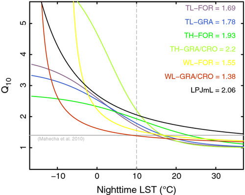
Above all discussions on the temperature sensitivity, our study shows that uncertainty in the approximation of the temperature sensitivity only contributes a small fraction to the overall RECO uncertainty. The temperature responses are mostly well constrained and overall model results from different temperature functions are very similar (Table S5). We point out that it is the uncertainty associated with limiting factors to the reference respiration rate that triggers considerable errors and remains a crucial issue.

Land cover types are aggregated to only two functional classes because it was crucial to divide the three climate classes first and the number of available sites remaining within each climate class restricts finer land cover separation. Nevertheless, accuracy in Re_std estimates is very high (R² = 0.78) and does not appear to be hampered by land cover aggregation. The LST_n response is smoothed across sites and land covers and temperature sensitivities do not vary much (Fig. 10). Forested and non-forested land covers are divided because of different EVI and LST_dif responses, but further separation of agricultural land is not significant with the data available. Using static land cover information (aggregated for the years 2001–2005) introduces errors for regions with extensive land cover change. Yet, we reduce uncertainties in the MODIS land cover product by aggregating classes to broader functional types.

More importantly, the coarse climate class stratification limits better Re standardization with sharper driver responses. Especially, the TH class spans a wide range from the tropical border in southern US to temperature-limited regions in Canada. Therefore, the phenological state within the growing season at a given temperature, T_ref, varies and thus the reference rate at T_ref does not standardize Re equally at each site. For example, Figure 4 g discloses a cloud of very high Re_std values around 20 °C LST, which follow an exceptionally high temperature dependency. This is an effect of T_ref being too early in the growing season and therefore confounds the standardization, which leads to unusually high Q₁₀ values for that biome (Fig. 10). Lower T_ref values, however, produce negative effects at the other end of the temperature range.

Parameter estimation is weighted by uncertainty, thus observations with small uncertainty have larger influence. This ensures that summer peak observations do not bias regression parameters, but accordingly they are predicted less accurately. Nonetheless, it is a general quality feature to achieve a reliable base-flow and reliable seasonal variation, rather than to match peak carbon efflux events. Residuals increase during the growing season, yet with no distinct bias (Fig. 9c). Further, we assume that autotrophic and heterotrophic shares are constant over the season, which is disputed (Falge et al., 2002; Davidson et al., 2006b). GPP and Ra decline in late summer, and Rh is amplified due to increased litter fall and precipitation. A partitioning of these processes by means of remote sensing appears currently not feasible. Also, RECO appears to be valid only for the equilibrium state since we do not account for feedback effects and slow soil carbon pools. We aim to establish a short-term monitoring tool for the current static state, for which it is not necessarily required to account for different carbon pools and soil turnover times (Migliavacca et al., 2011).

Besides these shortcomings of the RECO approach, Fluxnet measurements, especially of Re, contain considerable random and systematic errors. They can be attributed to limitations to the methodology and to differences in data processing. Random errors increase with magnitude of the flux (Richardson et al., 2006a; Richardson et al., 2008). Systematic errors arise from uncertainty in the partitioning methodology of NEE (Reichstein et al., 2005; Lasslop et al., 2010) and, more importantly, to advection losses at low-turbulence conditions, in spite of the applied u*-filtering (Aubinet, 2008; Williams et al., 2009). They mostly occur at nighttime and tend to produce underestimation in Re measurements (Massman & Lee, 2002; Baldocchi, 2003), which is important to point out since it might have contributed to the fact that the here presented study, as well as Jung et al. (2011), both result in Re estimates that are considerably lower compared to DGVM and literature values. However, the quantification and correction of systematic errors in the Fluxnet record is not trivial and critically remains a problem.

Moreover, Fluxnet sites represent major biomes with a sufficient number of sites to allow for stratified parameter estimates. A dense network is established among mid- and high latitudes at the northern hemisphere, but there is still a measurement gap for semiarid, arid, and tropical climates and for the southern hemisphere in general (Baldocchi, 2008). We only have data available for two sites in the tropics, where we can explain spatial variation to some degree, but predictors remain insignificant in accounting for seasonal variation (Samanta et al., 2012). Although it would be feasible in principle to extrapolate the model parameterization to the global scale, we therefore restrict our analysis to North America and Europe (where training sites are located). The carbon budget of the tropics is assumed to be close to neutral and the global terrestrial carbon sink is generally attributed to high-latitude extra-tropical areas (Pan et al., 2011), regions that are expected to be highly vulnerable to environmental change and also show large year-to-year variability (Canadell et al., 2007; Le Quéré et al., 2009).

DGVM comparison

We demonstrated that RECO has a negligible bias against Fluxnet Re observations and mean errors are smaller or comparable to previous studies. Furthermore, we show that Fluxnet towers are reasonably distributed over the range of annual sums calculated by RECO and LPJmL, which supports the assumption that incorporated Fluxnet data are representative and allow for upscaling. Moreover, RECO is able to reproduce large-scale spatial Re patterns disclosed by LPJmL, across all investigated biomes. Hence, we conclude that RECO is sufficient for up-scaling Re estimates to the continental-scale. Nonetheless, considerable differences exist in Re magnitudes between LPJmL and RECO, which merit further discussion.

Throughout this analysis, LPJmL simulates higher Re estimates compared to RECO and Fluxnet data. Here, we consider three possible explanations: (i) systematic bias in the Fluxnet measurement technique, (ii) inadequate parameterization of LPJmL, including the temperature sensitivity, and less likely, (iii) uncertainty due to scaling effects and climate and soil input data to LPJmL.

(i) Previous studies found systematic errors in the Fluxnet record due to advection losses to be significant. Jung et al. (2011) scale Fluxnet data to the global scale and calculate annual Re values 5–10% lower than previously thought, which they attribute to biased sampling and disturbance events. Kucharik et al. (2006) evaluate the IBIS DGVM, which employs the same temperature sensitivity as LPJmL, at Fluxnet sites and find a consistent overestimation in annual Re estimates at all three investigated sites of 16% to 29%. They associate errors with underestimation of observed nighttime Re at tower sites and also to a too pronounced temperature sensitivity of stem, root and leaf. Findings by Hanson & Amthor (2004) are similar; they find that the mean annual Re simulated by 10 independent models exceed observations by 27%. The above findings are in line with our results and thus we consider systematic errors in the Fluxnet record to contribute to the ‘shifted baseline’ between LPJmL and RECO. Yet, the associated uncertainty remains to be quantified.

Contradictory to this hypothesis is that model discrepancies show a distinct spatial pattern (Fig. 7c) and they are especially associated with high-level observations (Fig. 7d–f). It is particularly the boreal zone that stands out with a clear offset against Fluxnet data (Figs 8b, 9b, slope = 0.45 between Fluxnet and LPJmL), while mid-latitude continental regions are well in agreement.

(ii) In Figure 10, we show that the temperature sensitivity of LPJmL is generally higher than in RECO, which has a particularly strong effect at the upper temperature range. We consider this a possible reason that LPJmL shows higher estimates especially with high-level observations. The temperature sensitivity implemented in LPJmL is a well-known and commonly applied dependency, while many other DGVMs employ an even higher Q₁₀ of 2 (Friedlingstein et al., 2006). But recent studies suggest it could be overestimated (Mahecha et al., 2010), while practical conclusions for the ecosystem level remain difficult to draw (Reich, 2010; Graf et al., 2011). DGVM parameterization of the temperature sensitivity is critically important to study the climate change impact on the resilience of the carbon cycle and soil carbon stocks in particular (Jones et al., 2003). However, it is not only the temperature sensitivity that constraints Re simulations in LPJmL and biotic factors influencing the temperature dependence are as important (Davidson et al., 2006a; Bond-Lamberty & Thomson, 2010). Various process interactions between photosynthesis, precipitation and temperature and model assumptions, especially on turnover rates of soil carbon pools and soil parameters, determine Re simulations and conceal the mere dependency on temperature (Zaehle et al., 2005). But a mechanistic understanding of complex process interactions is still lacking (Davidson et al., 2006a). We argue that it is inadequate to associate model discrepancies with temperature sensitivities only. But it merits a further study to conduct a thorough parameter sensitivity analysis in order to identify those parameters in LPJmL that induce the apparent discrepancies. Moreover, LPJmL simulates higher global annual Re sums (129.68 ± 0.9 Pg C a⁻¹, 2000-2009) compared to recent estimates of 103 (Yuan et al., 2011), 96 ± 6.0 (Jung et al., 2011), and 119.6 Pg C a⁻¹ (Denman et al., 2007).

The finding that the here presented methods diverge fundamentally in the boreal zone is of critical importance to the modeling of the future resilience of the global carbon cycle. These high-latitude regions are expected to be specifically vulnerable to climate change impacts due to large carbon stocks and above average temperature increase (Dorrepaal et al., 2009; Bond-Lamberty & Thomson, 2010). Evidently, RECO cannot account for climate change impacts on slow carbon pools, but it provides a crucial measure to reveal current respiratory patterns and thus can help to calibrate DGVM estimates better, in order to increase our confidence in DGVM-simulated future climate change impacts.

We point out that the comparison of such intrinsically different models is only partly conclusive. For instance, comparing pixels of 1 km and 0.5° resolution involves errors due to scaling effects. RECO is trained and validated on Fluxnet data, thus it is clear that such a model will predict plot scale measurements better than a global process-based model not being calibrated to site-specific conditions. Gap-filling in MODIS and Fluxnet annual sums induce additional errors, but since the bias pattern is consistent across time aggregation, we neglect this point.

(iii) It remains difficult to assess uncertainty from climate input, but precipitation is generally the most uncertain variable. To test the associated uncertainty, we ran LPJmL with a competing precipitation data set (modified version of Oesterle et al., 2003), which generates a RMSE = 88 [g C m⁻² a⁻¹]. This is a considerable fraction of the 333 [g C m⁻² a⁻¹] between LPJmL and RECO.

Notwithstanding remaining shortcomings of the RECO methodology, RECO forms an operational, cross-validated, and unbiased approach to estimating continental-scale Re. It can readily be combined with existing GPP products (e.g., Sims et al., 2008) to calculate per-pixel NEE at 1 km and 8-day resolution. Since the steadily growing MODIS data pool now exceeds a decade of coverage, longer term trend analyses start to be feasible. Pending sufficiently accurate global estimates of terrestrial carbon fluxes, this study advances knowledge of local-scale spatio-temporal Re variability. We complement independent process-based estimates and reveal a critical gap among high-latitude regions. Underlying reasons that are contributing to such differences need to be further identified to reduce uncertainty in future projections of the global carbon cycle feedback to climate change impacts.