Modelling fatigue uncertainty by means of nonconstant variance neural networks
Funding information: Qatar National Research Fund, Grant/Award Number: NPRP-11S-1220-170112
Abstract
The modelling of fatigue using machine learning (ML) has been gaining traction in the engineering community. Among ML techniques, the use of probabilistic neural networks (PNNs) has recently emerged as a candidate for modelling fatigue applications. In this paper, we use PNNs with nonconstant variance to model fatigue. We present two case studies to demonstrate the developed approach. First, we model the fatigue life of cover-plated beams under constant amplitude loading, and then we model the relationship between random vibration velocity and equivalent stress in process pipework. The two case studies demonstrate that PNNs with nonconstant variance can model the distribution of the data while also considering the variability of both distribution parameters (mean and standard deviation). This shows the potential of PNNs with nonconstant variance in modelling fatigue applications. All the data and code used in this paper are openly available.
1 INTRODUCTION
Building a robust mechanical system with low maintenance cost requires accurate estimates of materials properties. Among these properties, metal fatigue continues to be challenging to estimate for several reasons. Metal fatigue is a complex phenomenon that is inherently uncertain due to a multitude of material properties and environmental and loading factors.1, 2 Wöhler3 developed the first deterministic S-N curve method, which remains to be among the most popular techniques used to characterize metal fatigue. The deterministic S-N curve is relatively simple and in agreement with many experimental tests. Another simple and well-known method for predicting fatigue life is the Palmgren-Miner linear damage rule.4 This approach is based on the “safe-life” method coupled with the rules of linear cumulative damage.
To produce more accurate estimates of fatigue life, several researchers proposed different deterministic techniques such as the use of energy models.5-7 Energy models for fatigue life prediction use either plastic energy, elastic energy, or the summation of both.
These approaches are deterministic and do not take into consideration the stochastic nature and uncertainties associated with fatigue. However, obtaining accurate estimates of the uncertainties associated with fatigue life is very important for estimating the durability and safety bounds of structural components subjected to cyclic loads.8 To address this issue, researchers developed deterministic1, 9, 10 and probabilistic11-13 approaches to account for these uncertainties. Randomness of the structural detail cannot be included in the deterministic approaches, which is one of their weaknesses. On the other hand, probabilistic approaches are fundamentally based on stochastics and are thus better suited to account for the inherent uncertainties of fatigue. One such probabilistic approach was proposed by Paolino et al.14 They used the Weibull distributions for constant and variable stress levels to build the probabilistic fatigue curve. Other approaches used the strain damage parameter to account for the uncertainty in the fatigue process.15 Another approach was proposed by Larin and Vodka16 to stochastically model the natural degradation of the materials properties and its effect on high cycle fatigue. Bayes' theorem with its great capability for probabilistic modelling has also been deployed to model fatigue. Many researchers used Bayes' theorem to develop probabilistic low-cycle fatigue life prediction methods.11, 13, 17 The maximum likelihood method18-20 is another probabilistic method that has shown the potential to minimize the time and the number of specimens required for testing and building a probabilistic S-N curve.
In recent decades, the fast-paced development of artificial neural networks (ANNs) and their ability to model linear and nonlinear relations using data without previous knowledge (i.e., without a set of rules or predefined heuristics) made them very attractive for fatigue applications. Researchers have used ANNs to evaluate the degradation of metallic and composite components21-23 and to predict fatigue life.24-26 For example, the modal properties of structures were used along with ANNs to identify loss of stiffness in structures and thereby indicate the presence of damage in the structure.27 Many researchers used ANNs to build S-N curves28 and constant life diagrams (CLDs).22, 29 Other researchers built an ANN to estimate the parameters of the Weibull distribution of the fatigue model.30 However, the previously mentioned methods (including ANN) considered the nonlinear behavior of the fatigue data but did not consider the nonlinearity of the uncertainty especially that the dispersion of the fatigue data is not constant throughout all the stress levels. Probabilistic neural networks (PNNs) with nonconstant variance have the advantages of both ANNs and probabilistic methods. This type of network has the capability of “learning” the data distribution and estimating both its mean and standard deviation. This means that the PNN will not only model the fatigue data; it will also model the uncertainty associated with it. PNNs also can preserve the uncertainty resulting from a small sample thereby reflecting the instability of statistical inferences.31 In general, S-N fatigue models show large uncertainty for fatigue life predictability at lower stress levels.32-34 Such uncertainty decreases as the stress increases; hence, the PNN with a nonconstant variance can be a powerful tool to accurately describe the changes of the stress scattering over the fatigue life cycle. Furthermore, using PNNs enables combining theoretical knowledge and the available experimental data by choosing the data distribution type. This feature allows building more realistic and robust fatigue models that take into consideration any physical constraints in the data.
Nashed et al.35 used PNNs with constant variance to model fatigue. PNNs with constant variance are suitable when the uncertainty in the data set is linear (or weekly nonlinear). The training process of a PNN with constant variance is not computationally demanding. Hence, using PNNs with constant variance when the uncertainty in the data set is weekly nonlinear is a good option. However, if the uncertainty in the data is nonlinear (as will be shown later), the PNN with constant variance will not provide a good representation of the data and the resulting PNN will lack accuracy; PNNs with nonconstant variance come forth in this case. To this end, this is the first work that uses PNNs with nonconstant variance to model fatigue. We present two case studies. The first case study concerns the fatigue of welded beams and the data that we will use is available in the literature. The second case study concerns vibration induced fatigue in process pipework due to flow induced forces. The data for this case study was obtained using finite element analysis and is also available in the literature.
The remainder of this paper is organized as follows. A review of machine learning, neural networks and PNNs is presented in Section 2. Section 3 presents the first case study: modelling fatigue in welded beams under cyclic loading. Section 4 presents the second case study: using PNNs to relate the vibration of pipework to the induced stress in the pipework. Conclusions for this work are drawn in Section 5.
2 MACHINE LEARNING
In this section, we present a brief overview of ANNs and PNNs.
2.1 Artificial neural networks (ANNs)
ANN is a class of computational tools inspired by the biological nervous system.36 The main processing unit in an ANN is called the neuron or perceptron. Each neuron has a weight assigned to it that is adjusted during the training process. ANNs have a great ability to learn linear and nonlinear relations to solve many problems without the need for a predefined set of rules. To create an ANN, the neurons are usually arranged in layers to form a multilayer perceptron (MLP). An MLP is composed of one (passthrough) input layer, one or more hidden layers and one output layer.36 Every layer, except the output layer, includes a bias neuron and is fully connected to the next layer. The network's error is calculated by the backpropagation algorithm during the training process which leads to the network's convergence towards the solution.
2.2 Probabilistic neural networks (PNNs)
PNNs are a subset of ANNs that have the additional capability of learning the distribution of the input data to estimate both the mean and the standard deviation of the network's output. Both types of networks (ANN and PNN) share a similar structure; that is, they both comprise of an input layer, hidden layers, and an output layer. Figure 1 shows a sample of the PNN's architecture. The ability of PNNs to learn data distribution makes them not only able to model the considered data but also account for uncertainty in the data and the model. Another advantage of PNNs is the generative property of the distribution. This feature makes PNNs an ideal candidate for solving regression and classification problems where the available data is limited. These useful properties make PNNs an attractive option for applications of fatigue and random vibration fatigue not only to assess failure limits but also to consider the physical variability of engineering components.
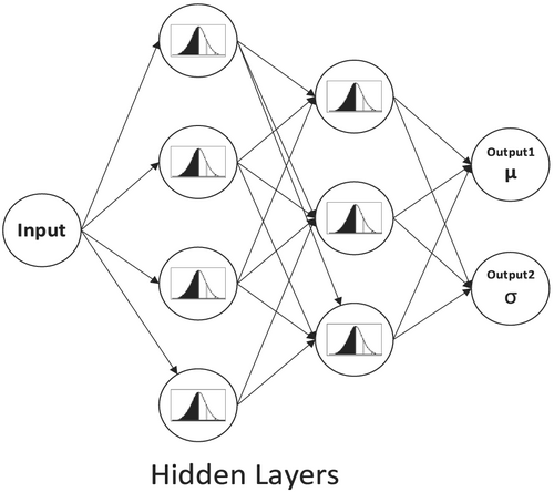
The structure of the PNN used in this research comprises a fully connected network that can model aleatoric uncertainty. The first layer is the input layer that has input neurons corresponding to the input data. Before commencing the building of the PNN, the data are normalized. For each data set, the normalization process is done by removing the mean and dividing by the standard deviation. This process normalizes the range of features of the input and output data sets. Then the input data would go through a set of hidden layers to learn the distribution of the input data to calculate both the mean and the standard deviation of the output data. Since the standard deviation is a positive number while the output of the PNN could be either positive or negative, the softplus function, defined as , is used for evaluating the data variability, that is, the standard deviation.
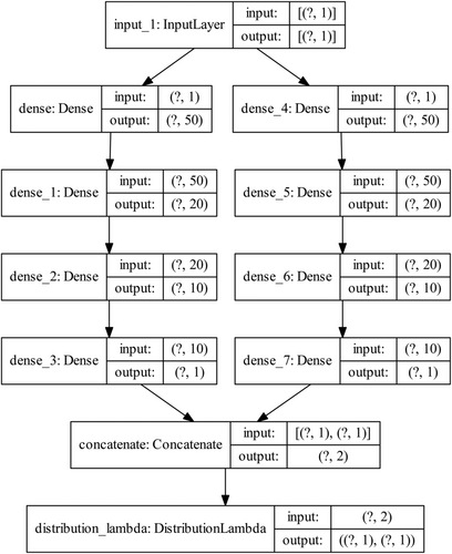
In this research, we allow the PNN's distribution parameter related to the standard deviation and the mean to depend on several layers between the input and the output as the relation between the input and output is nonlinear. Two stacks of hidden layers consisting of 50, 20, and 10 neurons were used in this research. One stack of layers is used to learn the mean of the input's distribution while the other stack is used to learn the standard deviation of the input's distribution. The concatenating layer concatenates the output of each stack in one layer. Then, the concatenating layer is connected to a DistributionLambda layer, which constructs the conditional probability distribution (CPD P[y|x, w]) and its standard deviation. TensorFlow Probability37 with Python38 and other toolboxes (namely, Pandas39 and Numpy40) were used to construct the PNN. The proposed topology of the PNN used in this research is shown in Figure 2. This topology was found to be stable during the training for the two case studies presented thereafter. In both case studies, the difference between the training and validation loss is small and does not increase during the training stage indicating the stability of the network.
To prevent overfitting of the network, three regularization techniques were used in this research. The first regularization technique that we used is L2 regularization, which constrains the weights of the neural network's connections. PNNs have hundreds of parameters that give them an incredible amount of freedom during the training phase. Hence, they can fit a huge variety of complex datasets. But this great flexibility also makes the network prone to overfitting the training data set. The L2 regularization technique works by punishing the network for using any extra parameters to fit the data. The second regularization technique we used is the dropout method.40 Here, at every training step, every neuron (including the input neurons but always excluding the output neurons) has a probability of being temporarily “dropped-out” of the network. The dropped-out neuron is entirely ignored during that training step, but it may be activated during the next step of the training process.
Furthermore, neural networks may also suffer from vanishing or exploding gradients during the optimization process which could prevent the network convergence to the optimal solution. The batch normalization technique is used here to reduce vanishing/exploding gradients during the training process. This operation simply zero-centers and normalizes each input, then scales and shifts the results using two new parameter vectors per layer: one for scaling and the other for shifting. For optimizing the network, the adaptive moment estimation (Adam) was used.43 This technique combines the ideas of momentum optimization44 and RMSProp.45 The momentum optimization part keeps track of an exponentially decaying average of past gradients while the RMSProp keeps track of an exponentially decaying average of past squared gradients. The NLL is used as a loss function to optimize the PNN with the coefficient of determination R2 computed as a measure of the PNN's performance.46 Finally, the Gridsreach method45 is used to search for best network parameters.
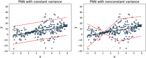
PNNs could be used to model data with constant and nonconstant variance (large heteroscedasticity). However, using constant variance with a problem where the heteroscedasticity is large enough will cause practical difficulties to estimate uncertainty accurately and will results with over or under estimation of data uncertainty. Figure 3 shows a simulated example for a set of data where the variance of the data changes significantly. The example illustrates the advantage of nonconstant variance PNN over the constant variance one. The constant variance PNN underestimates the uncertainty of data at range between 2 and 4 on the x-axis and overestimate data uncertainty between 1 and 2 on the x-axis of Figure 3. On the other hand, the nonconstant variance PNN accurately estimates the uncertainty over the entire range of the data. The difference between PNNs with nonconstant variance and PNNs with constant variance will be further illustrated in the second case study of Section 4.
The added accuracy that is provided by the nonconstant variance PNN comes at an added computational cost when compared with the constant variance PNN. Using nonconstant variance PNN to model a problem with low heteroscedasticity and small data size could result in noisy estimations since the nonconstant variance PNN was originally developed to focus on high variance data observations rather than optimal observation. Thus, it is recommended to use PNN with nonconstant variance for data with large heteroscedasticity and of reasonable size to estimate uncertainty properly. These useful properties of nonconstant variance PNNs make it an attractive option for applications of mechanical fatigue and random vibration fatigue not only to assess failure limits but also to consider the physical variability of engineering components accurately.
3 BEAM FATIGUE EXAMPLE
The data of cover-plated beams under constant amplitude loading are used to investigate the performance of nonconstant variance PNNs for modelling S-N curves and uncertainties in fatigue resistance. Figure 4 presents a schematic of the cover-plated beam with two configurations: welded (W) and unwelded (U) ends. The data have been collected from the work of Leonetti et al.13 although it was originally reported by Fisher et al.47
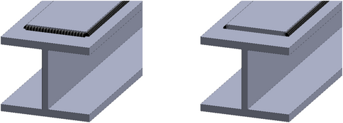
Table 1 provides a summary of the fatigue test data. The data in Table 1 are considered a “large sample” in agreement with the minimum requirements for fatigue tests as reported in the literature.48 The data are included in the appendix of Fisher et al.47 in the form of the tables cited in Table 1. Each table includes the specimen's name, stress range, minimum stress, the number of cycles at which the first crack was observed, and the number of cycles at failure. Leonetti et al.13 used these data to demonstrate the capability of Bayesian modelling to describe S-N relations in both low and high cycle fatigue more accurately than other deterministic methods. The main advantage of that technique over deterministic techniques is learning the data distribution. But the use of maximum likelihood method in that research13 considered the nonlinearity of one parameter (mean ) of the learnt distribution. The consideration of nonlinearity of both distribution parameters is a complicated process, which involves manually extracting the optimizing functions. Choi and Darwiche49 showed that probabilistic neural networks are more expressive than Bayesian networks since Bayesian networks do not use independence forms (e.g., causal dependence, etc.) that could improve their conciseness.50 PNNs have the potential to model applications that consider the nonlinearity of both distribution parameters (i.e., mean and standard deviation ). This capability not only allows modelling the data but also modelling the associated uncertainty. Here, we use PNNs with nonconstant variance to model fatigue in the beam fatigue data47 and to demonstrate the ability of this network to accurately model both the S-N curve and the associated uncertainty.
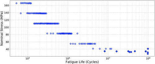
Figure 5 shows the beam fatigue resistance data used herein. The main observation is the change in data distribution during the transition from finite fatigue life (lower fatigue life cycle) to infinite fatigue life (over 107 cycles).
To process these data through PNN of Section 2.2, we first normalized the beam fatigue data as described earlier. Then the data were randomly split into training and validation sets with 80% and 20%, respectively. To increase the flexibility and robustness of the PNN, we not only increase the number of the hidden layers to maximize the maximum likelihood value (of Equation 1), but we also allow the PNN to learn both distribution parameters, that is, the mean and the standard deviation throughout its layers. This process allows the network to learn the data spread and to accurately estimate the uncertainty in the data.
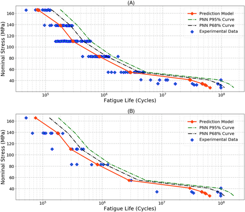
Figure 6 shows the PNN prediction of fatigue life against nominal stress for training and validation data. The figure also displays PNN modeling for aleatoric uncertainty associated with the fatigue data. The two curves for P68% (1-sigma) and P95% (2-sigma) demonstrate that the PNN with nonconstant variance can model the variability of fatigue life. Figure 6 also shows that the values of the standard deviation at high nominal stress gradually decrease up to around 50 MPa of nominal stress. Then, the standard deviation of the data quickly changes after that level. The coefficient of determination R2 for both training and validation is over 0.83. The variation of the standard deviation could not have been observed without the use of the PNN with nonconstant variance.
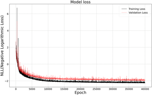
The convergence of the PNN in training and in validation is assessed using the NLL function defined in Equation 1. Using this loss function, the network is trained to maximize the likelihood between the network output and the experimental values. The training is run for 40,000 epochs as shown in Figure 7. In every epoch, the PNN of Section 2.2 runs through the entire training dataset, which gives the chance for every sample in the dataset to contribute to updating the hyperparameters of the PNN. Figure 7 shows the estimated NLL during the training and the validation against the epochs. Both training and validation loss in Figure 7 start at large values, then reduce into lower values at the end of the training process. The gap between training and validation loss stabilizes after nearly 25,000 epochs. These observations are indicators of a good network convergence without any signs of overfitting.
4 RANDOM VIBRATION OF PIPEWORK
Vibration induced fatigue in process pipework is the third reasons for all hydrocarbon releases in the UK North Sea.51 Oil and gas operators usually screen for this risk by measuring the vibration of pipework and discerning whether strain measurement and fatigue life calculations are required. In this subsection, we use PNNs to study the relationship between the vibration velocity of a pipe and the equivalent stress in the weld of the branch. This is the location that is most prone to experiencing vibration induced fatigue.
Figure 8 shows the generic model that was used in this paper. Vibration velocity and stress data will be generated through finite element analysis (FEA) using random vibration as an input excitation—this mimics the loading of flow-induced turbulence inside the pipe. The pipe is supported at its ends using rotational and translational springs to simulate different supporting conditions. The full data set along with further discussion of this example was provided by Shadi et al.52

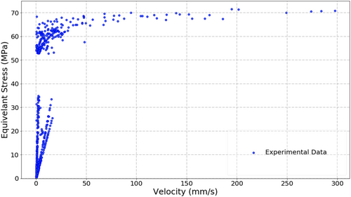
Figure 9 shows a plot of the vibration velocity and the equivalent stress. It is clear in the figure that the relationship is highly nonlinear. It is also clear in the figure that the equivalent stress data varies rapidly within a small range of vibration velocity, that is, 0 to 50 mm/s. The variations result in a large uncertainty in the equivalent stress within this range of velocity. Using data of such characteristics can be a serious challenge to implement machine learning approaches. Hence, we choose this set of data to demonstrate the ability of the proposed PNN with nonconstant variance in capturing such behavior.
4.1 Generated of FEA data
One model was created of the pipe setup shown in Figure 8. The model is composed of a 5″ SCH 40 carbon steel mainline that is connected to 25 cm and 2″ SCH 40 branch pipe using a 2″ × 5″ SCH 40 weldolet. The pipe, weldolet, and branch have a density of 7850 kg/m3, Poisson's ratio of 0.3, and modulus of elasticity of 200 GPa. The branch pipe supports a 5 kg valve (represented in the model as a point mass). The length of the mainline pipe is 0.3 m in the model. A fillet weld was added to join the mainline with the weldolet and another fillet weld was added to join the weldolet and the branch pipe.
The pipe was excited using the power spectral density (PSD) of a force that is generated from the flow of fluid. Riverin and Pettigrew53 measured flow-induced forces using different flow regimes and flow speeds. They characterized in-plane forces inside their pipes and showed that the flow-induced forces can be described using PSD curves and that the excitation frequency of flow induced forces does not exceed 100 Hz. We adopt their results in this work and use their PSD curves to excite the pipe of Figure 8. For the flow-induced excitation, two parameters will be changed: the liquid/gas ratios and the flow velocity.52 Four values of liquid/gas ratio were considered along with 16 flow velocities. Furthermore, the translational and rotational springs were varied as well to simulate different supporting conditions. Five sets of translational and rotational spring values were considered (Table 2). Based on all the previous information, the stiffness ratio for the simulated data was between 0.001 and 20. The total number of simulated models is 1025 (Table 3). The outputs of each model were the velocity of the valve in mm/s and the maximum stress in MPa in the fillet welds since this is the location most prone for fatigue failure.
| Translational support stiffness | Rotational support stiffness | ||
|---|---|---|---|
| (N/m) | (lb/in) | (N-m/rad) | (lb-in/rad) |
| 112.98 | 1 × 10³ | 1129.85 | 1 × 10⁴ |
| 5705.73 | 5.05 × 10⁴ | 57,057.34 | 5.05 × 10⁵ |
| 11,298.48 | 1 × 10⁵ | 112,984.83 | 1 × 10⁶ |
| 570,573.38 | 5.05 × 10⁶ | 5,705,733.88 | 5.05 × 10⁷ |
| 1,129,848.29 | 1 × 10⁷ | 11,298,482.93 | 1 × 10⁸ |
4.2 PNN for random fatigue pipework data
The topology of the proposed PNN to predict the velocity-stress relation is like the one mentioned in Figure 2. The network has one input layer with two stacks of hidden layers consisting of 50, 20, and 10 neurons. One stack of layers is used to learn the distribution mean while the other to learn the distribution standard deviation of the input data. The output layer concatenates the output of each stack in one layer. The output layer is also connected to a DistributionLambda layer. To reduce the probability of vanishing or exploding gradients at the beginning of the training, He initialization56 along with ELU activation41 are used. Furthermore, to reduce the probability of the gradient vanishing at late stages of the training, Batch Normalization is used. Again, the dropout method and the L2 regularization techniques are used to prevent overfitting.
In this case study, we use the vibration velocity as the training data and the equivalent stress as the target data. This is mainly motivated by the practicality of measuring the vibration velocity for pipework in operation. The vibration velocity and the equivalent stress data for the 0.3 m pipe are split into three groups based on the range of the stiffness ratio (SR = rotational support stiffness/translational support stiffness). The first group includes the stiffness ratios being less than or equal to 0.002. The second group includes stiffness ratios higher than 0.002 but less than 0.2. The final group includes stiffness ratios between 5 and 20. For each group, the data are divided into two parts: one for training and the other for validation. To test the proposed PNN in modelling the network uncertainties, we first use it to predict the data in individual groups and then for all the data together.
Figure 10 shows the equivalent stress prediction and the aleatoric uncertainty for each group of the data. The plots show the experimental data, resulting regression model and both P68% and P95% uncertainty boundary curves. The PNN flexibility is reflected in the ability to handle the data and the uncertainty variation associated with each individual group successfully.
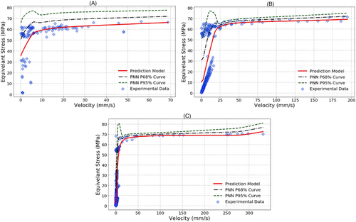
The resulting PNN model also achieves good coefficient of determination for all individual groups where R2 is shown in Table 4 for all the mentioned groups.
| Network | Validation data coefficient of determination R2 | ||
|---|---|---|---|
| SR ≤ 0.002 | 0.002 < SR ≤ 0.2 | 5 ≤ SR < 20 | |
| PNN nonconstant variance | 72% | 79% | 76% |
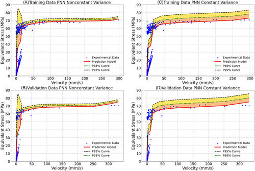
Next, the combination of all the data groups in one set is tested with both types of PNNs, that is, PNNs with constant and nonconstant variance. The previously described network procedures and parameters used for the individual groups are kept unchanged when working with the whole data. Figure 11 shows the results for both networks with training and validation data. The black dashed line represents the regression model while the blue and red dashed lines represent the P68% and P95% uncertainty boundaries. The results of Figure 11 show the ability of the proposed PNN with nonconstant variance to capture the equivalent stress variation better than the PNN with constant variance. The results show the variation to be accurately reflected although the stress varies intensely with small changes in the vibration velocity within the range 0 to 50 mm/s. The coefficient of determination for both training and validation datasets for the PNN with nonconstant variance was found to be >77% whereas that of the PNN with constant variance was around 74%, which demonstrates the superiority of the PNN with nonconstant variance.
The results presented in Figure 11 suggest that the proposed PNN with nonconstant variance can successfully model the nonlinear behavior of the data and accurately bound its uncertainty. The advantages of the proposed network are twofolds. First, the PNN with nonconstant variance can accurately identify the relation between the vibration velocity and the equivalent stress, which could not be achieved with a constant variance PNN. The second advantage is that the PNN with nonconstant variance can accurately estimate the uncertainty associated with the stress values relative to the vibration velocity. Those two advantages have practical importance for condition monitoring engineers. Some critical or costly decisions can be based on the proposed model predictions to avoid any unexpected fatigue failures or unnecessary costs resulting from early replacement of pipes or structural modifications to reduce the risk of fatigue.
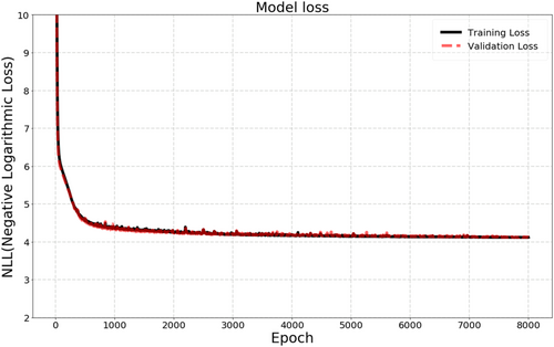
The learning progression of the PNN is measured using the previously defined NLL function. Figure 12 shows the estimated NLL against training epochs. It indicates a good fit for both training and validation loss where both curves decrease to a point of stability with a minimal gap between the two final loss values. Figure 12 also shows no signs of underfitting or overfitting in the network learning.
5 CONCLUSION
Fatigue displays stochastic behavior for multiple reasons such as material uncertainty, structural details, and environmental and loading conditions. Therefore, accurately accounting for the uncertainty associated with such behavior is important for the robust design, manufacture, and maintenance of mechanical components. Bayesian modelling demonstrated great aptitude to describe such behavior and account for uncertainties much better than many deterministic models. Bayesian approaches model fatigue data as a distribution, which allows the propagation of uncertainty through the model to quantify the uncertainty in the predicted fatigue life. However, such a process only considers the variability of the parameters of the corresponding distribution (usually the mean of the distribution). This means that the other parameter of the distribution (i.e., the standard deviation of the distribution) is considered constant during the modelling process. We propose using probabilistic neural networks (PNNs) with nonconstant variance to model such problems. Like Bayesian modelling, the PNN has the capability to learn the data distribution while also considering the variability of both distribution parameters (mean and standard deviation). This property allows PNNs not only to accurately describe the behavior of fatigue data but also account for uncertainty more precisely. In this paper, two case studies relating to fatigue applications are presented to demonstrate the proposed approach. The first case study concerns welded cover-plated beams under constant amplitude loading. The data for this case study is available in the literature and the objective is to obtain the S-N curve of the weld detail while accounting for the uncertainties of fatigue resistance. The proposed methodology captures fatigue life trends accurately and accounts for aleatoric uncertainty. The PNN further demonstrates its ability to account for the nonconstant variance in the data. For the second case study, we use the PNN to model the complicated probabilistic behavior of the random vibration and the equivalent stresses of a process pipework setup. The finite element method is used to simulate different flow and supporting conditions, thereby creating a large database for random vibration analysis. Random vibration of the pipework may lead to the development of fatigue cracks and failures. Thus, modelling such relationship is important for the integrity of process pipework. The data generated using the finite element method, is then used to train the proposed PNN to estimate the equivalent stress caused by flow-induced vibrations. The resulting probabilistic model achieves good results in terms of accuracy, robustness, and knowledge incorporation. The model is also a good example that demonstrates the capability of the presented approach to model both data and its uncertainty even when the relationship is highly nonlinear. The resulting PNN successfully describes the large variation of the equivalent stress in a narrow range of vibration velocity.
ACKNOWLEDGMENTS
Financial support for this research was graciously provided by Qatar National Research Fund (a member of Qatar Foundation) via the National Priorities Research Project under grant NPRP-11S-1220-170112. Open Access funding was graciously provided by the Qatar National Library.
Open Research
DATA AVAILABILITY STATEMENT
All the data and code used in this paper are openly available at Qatar University's Institutional Repository at https://qspace.qu.edu.qa/handle/10576/29984.


