Railway wheelset fatigue life estimation based on field tests
Funding information: In2Track3
Abstract
Field tests using an instrumented powered wheelset were performed to investigate fatigue damage accumulation in railway axles. Axle bending strains were measured and post-processed to obtain axle stress spectra. Statistical analyses were used to investigate the variations of axle stress spectra due to changes in railway operation parameters. The study indicates that measured axle stress spectra can be modeled using truncated normal distributions, where the large majority of measured stress amplitudes are lower than 50 MPa. Stress cycles at higher amplitudes are affected by operation parameters such as track design, number of switches and crossings, and whether the wheelset is in a leading or trailing position. Variations in the obtained statistical distributions of axle stresses have been used as input for fatigue life analyses. It was concluded that fatigue damage can potentially initiate on axles suffering from corrosion or small surface cracks/scratches.
1 INTRODUCTION
Railway axles are critical components of a vehicle's running gear. Their correct functioning is essential for travel safety. Railway axle maintenance is regulated by the European Standard EN 15313.1 According to this standard, non-destructive testing has to be performed on axles to detect possible cracks before those may reach a critical length, see Carboni.2 Inspection intervals running gear are usually scheduled depending on the mileage covered by the vehicle. However, such a scheduling approach does not account for the operational conditions the wheelset has been subjected to and the resulting status of the railway wheelset. This results in risks of trains being put out of service to perform unnecessary maintenance, or wheelsets subjected to extreme loads potentially being maintained too late. For the train operator, this results in higher maintenance costs, lower fleet availability, and potential safety issues.
To avoid the downsides entailed in current inspection practices, train operators are currently aiming at optimizing their maintenance intervals according to the observed conditions of their assets, see Cantini et al.3 This strategy is referred to as condition-based maintenance (Ben-Daya et al4), and it allows to postpone maintenance as long as the parameters used to monitor a certain asset fall in a “safe” range. This range can, for example, be prescribed by railway authorities or company practices, or determined by other forms of assessment. However, the fatigue design methods used in standards for railway axles vary significantly across the world, as shown by Makino et al.5 Moreover, to facilitate the adoption of a condition-based maintenance approach for railway axles, more knowledge regarding the statistical distribution of axle stress amplitudes is needed, as high stress amplitude values can have a negative influence on the axle fatigue life.
This gap has been partially filled by previous studies that investigated axle stress spectra. In Grubisic et al.,6 the operational loading of wheelset axles has been represented by cumulative frequency distributions (spectra) of service stresses. The total spectrum is obtained by summing up the contributions from the service stresses measured for trains running over stretches, respectively, characterized by straight tracks, curved tracks, and by the presence of switches and crossings. A “synthetic design spectrum” was also obtained by fitting a normal distribution over numerically computed stress levels. In Maglio et al.,7 bending stress spectra obtained by means of both numerical simulations and field tests have been used to assess the effects of wheel out-of-roundness (OOR) and rail roughness on the increase in axle stress magnitudes. It was shown that, for the studied cases, the increase in axle stresses due to rail roughness could overcome the increase in axle stress due to the degradation of the wheel tread geometry.
In other studies, measured or simulated axle stress spectra have used to perform fatigue analyses: in Wu et al.,8 a spectrum made of five blocks aimed at representing the stress distribution in the axle under different operational conditions was used to estimate the effects of a decrease in fatigue limit due to foreign object damage on the axle. Wu et al.9 used a stress spectrum to perform a stepwise fatigue assessment methodology where a safe life assessment step is followed by a damage tolerance analysis. In Nahlik et al.,10 a load spectrum was obtained by dividing measured bending amplitudes in 36 blocks depending on the dynamic load coefficient (i.e., the ratio between static load and measured load). The spectrum was then used to estimate the residual lifetime of the axle depending on the presence of detected or undetected cracks based on linear elastic fracture mechanics as well as by accounting for the retardation effect due to the plastic zone at the crack tip. In Mädler et al.,11 the residual lifetime of wheelset axles was estimated by carrying out an experiment with a test rig. The load history was derived from a load spectrum consisting of 17 block loads. In Beretta et al.,12 stress spectra obtained from field measurements have been used in a probabilistic fatigue damage assessment to determine the risk of fatigue failure of high-speed and freight train axles during service. The load spectra, which represented different service conditions, were used in Monte Carlo analyses resulting in a safety factor for a target reliability against fatigue.
The investigations in the above-mentioned works were mainly focused on variations in residual fatigue lifetime based on pre-determined axle stress spectra. However, a remaining question is related to the effects of variations in operational conditions on such spectra. In the present investigation, stress spectra are not only obtained as the cumulative distribution of bending stress values throughout the whole duration of a field test. Instead, also the different contributions to the spectra given by the passage over some specific sections of the railway network are analyzed. These sections are chosen depending on some operational parameters such as speed limits, number of curves, switches, and crossings. This allows to account for the variations in measured stresses due to the different operational conditions that can occur during operations on a stretch of track.
In this work, data in terms of bending strains have been gathered using the instrumented telemetry system described in Maglio et al.7 The system has been installed on a powered wheelset located at one end of a regional train. The train operates both on high-speed main railway lines (with a speed up to 200 km/h) as well as on single-track regional railways in Sweden. Stress spectra have been collected by the telemetry on-board computer unit between February 2019 and November 2020. More information about the field test is given in section 2 of the present work.
Axle bending stress spectra measured on different track sections have been used to estimate statistical distributions of axle stresses. Spectra obtained directly from field tests as well as spectra estimated from statistical distributions have been used as input to fatigue life analyses. In these analyses, different Wöhler (Stress-Number) curves were used to account for the influence of variations in axle surface conditions. Moreover, the reduction factors applied to the fatigue limits in the Wöhler curves have been compared to the effect of surface cracks of different lengths.
The obtained statistical distributions of axle stresses can be used to predict the stresses that have been experienced in service, thus allowing the train operator to adopt a predictive maintenance approach. Fatigue analyses may help in identifying threshold levels in axle surface conditions at which precautions need to be taken to avoid failures. Based on the results derived under different operational conditions, the planned maintenance can be scheduled to an earlier or later occasion, and priority can be given to wheelsets where the estimated residual fatigue lifetime is more critical. This would result in a more efficient use of resources for the train operator, as well as in more flexibility in the usage of the fleet.
2 FIELD TEST
2.1 The telemetry system
The telemetry system used in the field test monitoring stresses at a specified section of an axle was SmartSet®, developed by Lucchini RS. The telemetry system, which is described more in detail in Cantini et al.3 and Maglio et al.,7 consists of strain gauges and a telemetry module installed on the axle body, as well as of a data acquisition computer mounted on the vehicle body. In the present installation, two telemetry modules (each consisting of two full strain gauge bridges capable of measuring strains due to axle bending) are placed on the axle of a powered leading wheelset at a distance of 80 mm from the wheel seat, where the effect of the stress concentration is negligible. The telemetry module receives power from the train power supply via an induction power head that is installed on the gearbox frame. The power head generates an alternating current on the inductive coil that is installed on the axle and directly connected to the telemetry module. The locations of these components on the instrumented axle are indicated in Figure 1.
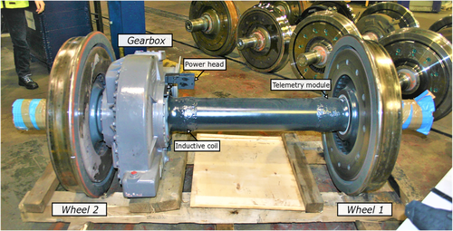
The telemetry module acquires data from the strain gauges and processes the signals according to a rain flow count algorithm. For each strain cycle identified by the algorithm, strain mean values and amplitudes are stored in matrices. Measured strains can then be easily converted into stresses. A Global System for Mobile Communications (GSM) antenna transfers matrices to a remote server when the train is at specific Global Positioning System (GPS) locations. This allows to relate measured stress spectra to traffic on specific sections of the network and thus to assess the influence of track quality on measured axle stresses.
The instrumented train is an electric multiple unit of type Coradia Duplex produced by Alstom and operated by the Swedish passenger train operator SJ. It consists of two or three double-decker coaches, and it can operate in both running directions at a maximum speed of 200 km/h. The axle load acting on the instrumented wheelset is around 18.25 tonnes. The end of the train where the instrumented wheelset is mounted is reserved for the driver and electric equipment. Consequently, the static load acting on the axle does not vary significantly during operation.
2.2 Axle stress spectra
Measurement data collected by the telemetry system in the form of strain matrices have been converted into stress matrices. Data gathered while the instrumented wheelset was traveling between Gothenburg and Skövde are shown in Figure 2. To facilitate the comparison of measurements for stretches of different lengths, results have been normalized and plotted in terms of “cycle ratio.” This ratio has been obtained by dividing the number of cycles falling within a stress amplitude bin with the total number of stress cycles measured during a given train ride. Moreover, cycles with measured stress amplitudes below 20 MPa have been removed from the plots as these are mainly due to oscillations in the voltage of the telemetry system.
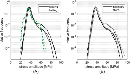
In Figure 2A, stress amplitudes are compared for some measurements performed when the instrumented wheelset is in leading or in trailing position. As the train can travel in both directions and as the instrumented axle is located at one end of the train, the instrumented wheelset can either be the very first or the very last wheelset to negotiate curves and switches when the train is running. From Figure 2A, it is possible to notice that larger stress amplitudes (in the order of 70 MPa to 90 MPa) are registered when the instrumented wheelset is in leading position. This is due to the fact that the first wheelset in the train suffers from higher wheel–rail contact forces (see Andersson et al.),13 which affects the measured stresses. As higher stresses can have much more detrimental effects from a fatigue life perspective, the work presented in this paper will be based on measurements obtained when the instrumented wheelset is in the leading position.
Figure 2B compares stress amplitudes (as obtained from the matrices) and equivalent SWT stress amplitudes for the three curves marked as “leading” in Figure 2A. It is possible to see that stress spectra consisting of SWT amplitudes are shifted about 1 to 2 MPa towards higher values. Although this increase in stresses is not expected to contribute significantly to the accumulation of fatigue damage in the axle, SWT equivalent amplitudes will be used in this work to properly account for the effect of mean stresses
2.3 Statistical interpretation of stress spectra
Stress spectra obtained from different measurements performed between May 2019 and November 2020 for two different sections of the Swedish rail network (Gothenburg–Skövde and Skövde–Hallsberg) are plotted using thick dashed red lines in Figure 3A and 3B. During these measurements, the instrumented wheelset was placed in leading position with respect to the train traveling direction. These track sections, which have comparable lengths, are part of “Västra Stambanan,” a mixed traffic railway line connecting Gothenburg and Stockholm. Being part of the same line, the two sections are expected to undergo similar maintenance procedures and have similar levels of rail roughness.
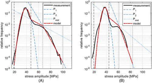
From Figure 3, it can be noticed that the most frequently measured equivalent stress amplitudes fall between 35 MPa and 40 MPa, regardless of the route that the train is traveling on. This is expected as most of the equivalent stress amplitudes are only influenced by the (quasi-)static load acting on the axle, which depends on the weight of the train and not on the specific route. Moreover, Figure 3 shows that, as the equivalent stress amplitudes increase, their relative occurrence drops significantly, particularly for equivalent stress amplitudes larger than 60 MPa. It can be noted that the relative occurrence of equivalent stress amplitudes starts its rapid decrease at lower amplitude levels when the train is traveling on the route Skövde–Hallsberg (see Figure 3B) than on the route Gothenburg–Skövde (see Figure 3A). This cannot be explained by differences in track quality, as the two routes are expected to have similar speed limits and maintenance statuses. Instead, variations in relative occurrences of equivalent amplitudes may be due to differences in track design. These differences are summarized in Table 1, which shows the relative amounts of switches, crossings, and narrow curves on the two routes.
| Railway line | Gothenburg–Skövde | Skövde–Hallsberg |
|---|---|---|
| Length of the line (km) | 143 | 109 |
| Number of switches and crossings per km | 0.59 | 0.39 |
| Number of curves per km: | ||
| with curve radius < 1000 m | 0.43 | 0.04 |
| with curve radius < 700 m | 0.29 | 0 |
The amount of switches and crossings per kilometer for the route Skövde–Hallsberg is about 50% higher compared to the route Gothenburg–Skövde. Moreover, the occurrence of curves with radius lower than 1000 m of track is more than 10 times higher for the route Gothenburg–Skövde than for the route Skövde–Hallsberg. The route Gothenburg–Skövde is also characterized by a significant amount of sharp curves with radius lower than 700 m, which instead are not present on the Skövde–Hallsberg route. As switches and crossings as well as curves (and transitions curves) cause variations in the geometry of the track, leading to increased wheel–rail contact forces and axle stresses, they are likely reasons for the increased occurrence of higher equivalent stress amplitudes on the Gothenburg–Skövde route.
It should be pointed out that this investigation does not account for the variations in wheel OOR or rail roughness that have been observed during the measurement period. However, a study in Maglio et al.7 has shown that the increase in axle bending stress amplitudes due to increased wheel OOR (up to 120 μm in peak-to-trough ovality) or due to a deterioration in rail surface roughness (up to 0.5 mm in peak-to-trough rail vertical roughness) is only in the order of a few megapascals. As a consequence, it is reasonable to expect that small variations in wheel OOR and rail roughness are not significant contributions to the variations in axle stress amplitude spectra.
Weather conditions and track stiffness were not monitored during the field test. However, as the measurements were performed over a period of 22 months, it can be expected that seasonal variations in weather and track stiffness are evened out throughout the different measurements for the same track section.
To obtain a model of the stress spectra that can be used to predict the wheelset loads during operations along a certain route, it is noted that the measured stress spectra are characterized by a peak in the interval between 35 MPa and 40 MPa and by a drop that generally occurs at stress levels higher than 60 MPa. In between, there is a section characterized by a slower decline or by a plateau in the frequency of measured stress levels.
Two normal distributions, denoted P1 and P2 in Figure 3, have been fitted to the first and last parts of each stress spectrum (each characterized, respectively, by a peak and by a drop in frequency of measured stress magnitudes). Consequently, the two normal distributions P1 and P2 are only fitted to the parts of the stress spectra located, respectively, to the left and to the right of the central plateau. The way the normal distributions P1 and P2 are fitted to the measured spectra is shown in Figure 4.
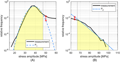
As seen in Figures 3 and 4, the two normal distributions deviate significantly from the measured curve (black solid line) towards the center of the spectra. In order to account for that, the distributions P1 and P2 have been truncated before the difference in relative frequency between the measured stress spectra and the statistical distributions reaches 50%. The SWT stress amplitude value at which the difference between P1 and P2 and the measured spectra exceeds this threshold is shown in Figure 4 with red vertical segments ending with circles. As stress spectra are stored by the telemetry in stress bins which are 2.8 MPa wide, the truncation occurs at the bin closest to the one where the threshold is exceeded. After the truncation procedure has occurred, only the untruncated parts of normal distributions P1 and P2 (highlighted in yellow in Figure 4) are used to model the load spectra.
In Figure 3, the stress amplitude levels at which P1 and P2 have been truncated are marked with black vertical dashed lines and black vertical dotted lines, respectively. The part of the stress spectra located between the two truncated normal distributions (roughly corresponding to stress amplitudes between 45 MPa and 60 MPa) has been modeled by a straight line in the semilogarithmic diagrams and is denoted Pmid. The truncated distributions P1, Pmid, and P2 form the full stress spectra model. In Figure 3, it is indicated by dashed red lines.
The obtained models of stress spectra can be useful in the design of wheelset components as well as in maintenance planning, as service loads in real operations are often higher than the ones that can be determined according to the procedures suggested in the standards such as EN 13013–1,15 see Grubisic et al.6
3 FATIGUE ANALYSES
Both the stress spectra obtained from the measurements and those obtained from the statistical models can be used to predict the residual lifetime of the wheelset. The analyses performed in this work will be focused on axle fatigue, but the method can be applied to other wheelset components by transforming to relevant service stresses.
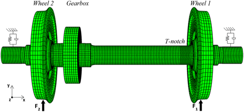
In the present field test, stress amplitudes have been derived by measuring axle strains in a location where the effects of stress concentrations are not present. However, stresses will increase towards the fillet radius located below the wheel seat, also known as T-notch, where axles are most commonly cracked, see Lundén et al.16 and Madia et al.17 To account for the state of stress in the vicinity of the T-notch, a three-dimensional finite element (FE) model of the instrumented wheelset was used, see Figure 5. The model has 788,568 degrees of freedom and is loaded with two unit forces F1 and F2 applied on the nominal circles of the two wheels and acting along the vertical direction. The vertical displacement of the wheelset is limited by the primary suspension, which is modeled as two pairs of springs and dampers. The springs stiffness is 2 MN/m, and the dampers viscous coefficient is 20 kNs/m. The material properties and the geometry of the model are described in detail in Maglio et al.18 A static analysis showed that the maximum bending stress value at the T-notch is 1.26 times higher than at the cross section of the axle where the strain gauges are mounted. As a consequence, a static stress concentration factor Kt = 1.26 has been used in the present work for the T-notch.
3.1 Fatigue life relationship
In order to assess the fatigue life of the axle under different operational conditions, reduction factors to be applied to the Wöhler curve (S–N curve) were estimated from test data and modified according to the method of Juvinall et al.19 as described in Dowling et al.20
The axle of the instrumented wheelset is made of EA1N steel. According to the European Standard EN 13261,21 the ultimate tensile strength ) of that material falls in the range between 550 MPa and 650 MPa. In the present study, = 600 MPa has been used. Fatigue limits for axles made of EA1N steel were obtained from full-scale tests in Cervello.22 For such an axle with a surface roughness in the range 0.8 to 1.6 Ra (presuming to correspond to a machined surface), an average fatigue limit of 248 MPa (with a standard deviation of 34 MPa) was estimated for 107 stress cycles. This corresponds to a fatigue limit of 181 MPa for 2.5% probability of failure. Calculations in this study are performed for axles in service and are therefore mainly aimed for maintenance planning. Therefore, the average fatigue limit is used, as it gives a more realistic estimation of the residual life of the axle. The fatigue limit for 2.5% probability of failure should be used when designing the axle, as a larger safety margin should be aimed for.
According to Juvinall's theory, the Wöhler curve can be expressed as a straight line in a semilogarithmic stress-cycles chart between the fatigue limit, , and the stress amplitude corresponding to a fatigue life of 1000 cycles. To match the experimental data in Cervello,22 the fatigue limit was set at 107 cycles.
Fatigue life analyses have been performed for the T-notch using as input both the stress spectra obtained from the measurements and those obtained from the fitted statistical distributions. In this paper, results obtained for the stretches Gothenburg–Skövde and Skövde–Hallsberg are presented, but the approach has also been applied to analyze other stretches of the Swedish railway network.
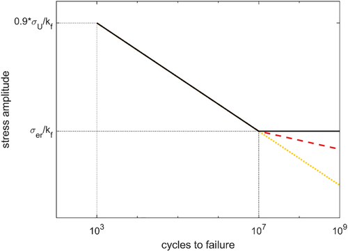
In our analyses, three different fatigue damage calculation algorithms have been applied. In the first one, it is assumed that stress cycles whose equivalent SWT amplitudes fall below (i.e., the reduced fatigue limit for 107 cycles) do not cause any fatigue damage. This is the least conservative design approach. In the second approach, it is assumed that all cycles cause the same amount of fatigue damage that would be predicted by simply prolonging the slope of the S–N curve for fatigue lives higher than 107 cycles. This is the most conservative approach and may result in an over-conservative design and fatigue life estimations. In the third approach, it is assumed that the Wöhler curve continues after 107 cycles with a reduced slope (one third the slope of the S–N curve between 103 and 107 cycles). The Wöhler curves resulting from these assumptions are sketched in Figure 6.
3.2 Effect of operational conditions
The Wöhler curves represented in Figure 6 have been adopted to estimate axle fatigue life using the stress spectra (with SWT correction) obtained from the telemetry measurements as well as the spectra obtained from the statistical models. When analyses are based on the statistical distributions, a Monte Carlo approach is used. Here, stress amplitudes are not extracted from measured spectra but derived from random realizations of the model distribution built up from the truncated distributions P1, Pmid, and P2 according to their pertinent (truncated) probability density functions. Realizations are allocated to one of the three truncated distributions depending on their cumulative probability. This implies that, for example, more realizations are generated based on P1 than P2. Each realization in the Monte Carlo approach corresponds to a SWT stress amplitude value.
In order to account for a large variety of possible maintenance conditions, in particular relating to the axle surface conditions, different values for the surface roughness coefficient have been applied when reducing the Wöhler curve. The magnitude of affects the fatigue limits for 107 cycles as shown by dotted gray vertical lines in Figure 7.
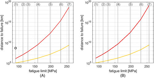
Figure 7 shows that the estimated axle fatigue life is strongly dependent on the reduction factors applied to the Wöhler curve as well as on the adopted fatigue life algorithm. In contrast, despite the two railway stretches generating different axle stress spectra, no large differences are visible between Figure 7A and 7B. This is due to the fact that the largest majority of stress cycles correspond to the part of the stress spectra represented by the probability distribution P1 which does not differ significantly between the two running cases. Even if the equivalent stress amplitudes modeled by P1 are relatively low in magnitude, their relative frequency is so high that they contribute for the largest share of the total damage D (see equation 7) when it is assumed that all stress cycles contribute to the accumulation of fatigue damage (i.e., in the cases represented by the red and yellow curves in Figure 7). The black circle shows that, if it is assumed that stress amplitudes below the fatigue limit are presumed not to generate any fatigue damage, fatigue failure can only occur for axles with very critical surface conditions. This hypothesis is non-conservative and unrealistic, and should not be adopted for maintenance planning.
Moreover, it can be concluded that there are no large differences in predicted fatigue lives between measured and simulated stress spectra. This indicates that approximating stress spectra using statistical distributions leads to a low error, see the following section.
3.3 Sensitivity analyses
As Figure 7 is plotted in semi-logarithmic scale, it might be difficult to notice small variations between the different curves. Table 2 has been added to clarify the differences in expected axle fatigue lives between the two stretches as well as between the two modeling assumptions for stress spectra. In the results shown in Table 2, the axle surface is assumed to be fine ground, and the Monte Carlo analyses have been performed with 107 trials.
| Expected distance to axle failure (km) | Difference in expected distance to failure between models | |||
|---|---|---|---|---|
| Model for stress spectra based on | Same S–N slope | 1/3 slope | Same S–N slope | 1/3 slope |
| Gothenburg–Skövde | ||||
| Telemetry | 49*108 | 65*1013 | 4.1% | 3.1% |
| Monte Carlo | 47*108 | 63*1013 | ||
| Skövde–Hallsberg | ||||
| Telemetry | 53*108 | 117*1013 | 3.7% | 14.4% |
| Monte Carlo | 51*108 | 102*1013 | ||
Table 2 confirms that the statistically derived stress spectra introduce differences in estimated distances to axle failures lower than 15% and in many cases lower than 5%. It can be noticed that the differences in expected axle fatigue life between the two track sections are strongly dependent on the hypotheses on the slope of the Wöhler curve (i.e., on whether the slope is reduced or not after 107 cycles). Indeed, if it is assumed that the slope of the Wöhler curve does not change, the expected axle life differs about 8% between the two stretches, while it differs of over 40% if the S–N curve slope is reduced to one third after 107 cycles. This is due to the fact that in the latter case stress cycles with lower amplitudes generate a lower amount of fatigue damage. Thus, less fatigue damage is accumulated for a stretch where registered stress amplitudes are lower (such as Skövde–Hallsberg).
Monte Carlo analyses whose results in terms of fatigue life are shown in Figure 7 have been performed for 107 trials. However, it is possible to obtain robust results even with significantly lower amounts of trials. Figure 8 shows the difference in expected axle fatigue life computed using the stress history from the telemetry or the Monte Carlo approach as a function of the amount of trials.
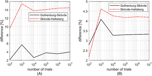
Figure 8 shows that the error obtained using the Monte Carlo method tends to stabilize after some 104 to 105 trials. This means that reliable fatigue life analyses can be made with a low computational cost (a Monte Carlo fatigue analysis with 106 trials and accounting for the three different fatigue algorithms requires around 3 min to be performed on an Intel i7 processor).
3.4 Effect of overloads
The stress spectra and the statistical distributions in Figure 3 show that a clear majority of cycles are characterized by stress amplitudes lower than 50 MPa. The occurrence of those stresses is modeled by the statistical distribution P1, see section 2.3. Moreover, the results from fatigue life analyses summarized in Table 2 and discussed in section 3.2 indicate that cycles with lower stress amplitudes actually generate the largest contribution to fatigue damage—how large this contribution is depends on the assumptions made on the slope of the Wöhler curve, see section 3.1.
The share of fatigue damage caused by the three statistical distributions P1, P2, and Pmid (see Figure 3) in the fatigue life analyses performed with the Monte Carlo method is shown in Table 3. The analyses are related to the stretches Gothenburg–Skövde and Skövde–Hallsberg. The axle surface was supposed to be machined, a condition that corresponds to the vertical lines marked with (5) in Figure 7.
| Railway lines | Constant S–N slope | 1/3 slope after 107 cycles | ||||
|---|---|---|---|---|---|---|
| P1 | Pmid | P2 | P1 | Pmid | P2 | |
| Gothenburg–Skövde | 79.2% | 17.1% | 3.7% | 39.3% | 34.1% | 26.9% |
| Skövde–Hallsberg | 81.2% | 16.9% | 2.0% | 54.4% | 34.6% | 11.0% |
It can be noticed that stress cycles with relatively low amplitudes (i.e., those modeled by the distribution P1) account for between 39% and 82% of the accumulated damage depending on track quality and assumptions on the fatigue algorithm. Stress amplitudes falling under the distribution P2 can reasonably be classified as overloads. From Table 3, it can be noticed that overloads can significantly affect the fatigue life of the axle if the slope of the Wöhler curve is reduced after 107 cycles, since 11% to 27% of the fatigue damage is generated by these loads. If the slope of the S–N curve is instead presumed to be unaffected by the fatigue limit, overloads only account for 2% to 4% of the fatigue damage. In this more conservative approach, indeed, stress cycles at lower amplitudes generate more fatigue damage.
To investigate this topic more in depth, fatigue life analyses featuring only stress cycles from the untruncated normal distribution P1 as input in the Monte Carlo analyses have been performed. The difference between the expected axle fatigue lives including the three distributions P1, Pmid, and P2 and the fatigue analysis featuring the untruncated P1 distribution is plotted as a function of the axle surface conditions in Figure 9, and fatigue limits as in Figure 7. The Monte Carlo analyses have been performed with 107 trials and are related to the stretches Gothenburg–Skövde and Skövde–Hallsberg. The percentages of Figure 9 are based on the expected fatigue life if all three distributions are accounted for.
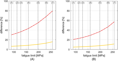
Figure 9 shows that cycles with higher stress levels are less significant if the slope of the S–N curve is not changed. This is, as also remarked above, due to the fact that stress cycles at lower amplitudes generate more fatigue damage if the slope of the S–N curve is unchanged.
Not accounting for the probability distributions Pmid and P2 leads to a larger overestimation of the fatigue life for the stretch Gothenburg–Skövde than for Skövde–Hallsberg. This is due to the generally higher stress levels on the first stretch. Overall, under the assumption that the slope of the Wöhler curve is reduced after 107 cycles, neglecting cycles with higher stress levels leads to a large overestimation of the fatigue life (between 20% and 80%).
3.5 Effect of small surface cracks
Axle structural integrity is reduced by the presence of small surface defects (cracks) that may not be detected during scheduled inspections. In Beretta et al.,25 the effect of corrosion by rainwater on the S–N diagram of A1N steel was studied by means of fatigue tests on cylindrical specimens.
Equations (9) and (19 have been used to obtain the radii of small semi-circular surface cracks that would generate different reduced fatigue limits for the axle. Then, axle residual lives for the two stretches Gothenburg–Skövde and Skövde–Hallsberg have been computed for the above-mentioned reduced fatigue limits and for different assumptions on the slope of the Wöhler curve. Estimated fatigue lives for axles affected by small semi-circular surface cracks were thus obtained according to the theories of Murakami and El Haddad, see Figure 10. These analyses do not account for the variation in stress intensity factors due to crack growth, and the adopted equations are only valid for small cracks. As a consequence, results are only indicative and intended to be used as an aid in maintenance planning.
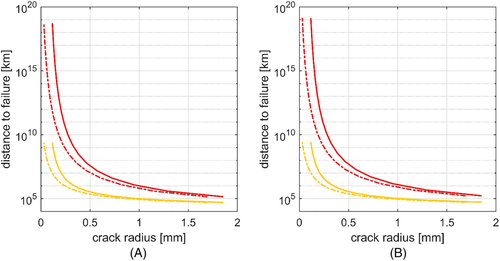
Figure 10 shows a good match between the results obtained with Murakami and El Haddad theories. Again, the expected fatigue life changes significantly depending on the assumptions made on the slope of the Wöhler curve and on the adopted fatigue algorithm.
4 CONCLUDING REMARKS
Bending stress spectra of railway axles have been derived from field tests. A method to obtain statistical descriptions of these spectra using truncated normal distributions has been presented. Field test and statistical stress spectra have been used as input to fatigue life analyses accounting for different assumptions on the Wöhler curve. Results show a good agreement between fatigue lives obtained from measured and statistically described stress spectra. Moreover, it was shown that Monte Carlo-based fatigue life predictions converge after a relatively low amount of trials. Results in terms of expected fatigue lives are heavily dependent on the hypotheses made on the reduction of the Wöhler curve at lives >107.
The derived statistical stress amplitude distribution provides an objective categorization of the track section quality with respect to wheelset loading. The developed fatigue assessment approach can also be used to predict the estimated residual fatigue lifetime of wheelset components, contributing to the adoption of a condition-based maintenance approach. In future work, efforts will be made to link the parameters of the statistical distributions used to model stress spectra with measured track conditions (e.g., track geometry deviations, amount of transition curves, and of switches and crossings).
ACKNOWLEDGMENTS
The current work is part of the activities within the Centre of Excellence CHARMEC (CHAlmers Railway MEChanics, www.chalmers.se/charmec). Parts of the study have been funded from the European Union's Horizon 2020 research and innovation program in the project In2Track3 under grant agreement No. 101012456.
NOMENCLATURE
-
-
- projected area of surface defect
-
-
- crack length
-
-
- accumulated fatigue damage
-
-
- crack geometry factor
-
-
- Vickers hardness
-
-
- crack stress intensity factor
-
-
- notch stress intensity factor
-
-
- S–N curve reduction factor
-
-
- number of stress cycles to failure
-
-
- probability distribution
-
-
- stress amplitude
-
-
- Smith-Watson-Topper (SWT) equivalent stress amplitude
-
-
- reduced fatigue limit for rotating bending
-
-
- threshold stress for crack growth
-
-
- maximum stress value
-
-
- ultimate tensile strength
Open Research
DATA AVAILABILITY STATEMENT
Research data are not shared.


