1 INTRODUCTION

Multicellularity allows an organism to divide tasks between cells, creating a complex soma with a much wider range of functions than single-celled organisms can achieve (Grosberg & Strathmann, 2007; Knoll, 2011). It also permits large body size, which may help in predator avoidance (Boraas, Seale, & Box horn, 1998; Kapsetaki & West, 2019) and be subject to other types of selection to become large, including metabolic scaling (White et al., 2019) and intraspecific competition (Kingsolver & Pfennig, 2004; Pettersen, White, & Marshall, 2015). However, creating and maintaining the soma of a multicellular organism is not a trivial task. This requires cooperation between their individual cells, where somatic cells forgo passing their genetic material to the offspring, and they divide only to maintain organismal functions. From a single somatic cell's perspective, if the benefits of cooperating outweigh self-replicating, this can still be advantageous (Goldsby, Knoester, Ofria, & Kerr, 2014; Libby, Conlin, Kerr, & Ratcliff, 2016). But even if somatic cells “aim” to cooperate, they inherit their genomes from germline cells that have unlimited dividing potential, and the adjustments required to make cells a differentiated part of a somatic tissue may not always function flawlessly. Uncontrolled growth (cancer) is one problem (Aktipis et al., 2015), and since tumours typically only arise when several mutations have occurred in the same cell lineage, the number of “permitted” cell divisions has evolved to be limited (Campisi, 2013; Maciejowski & de Lange, 2017; Sager, 1991). Other aspects of somatic maintenance include strategies such as damaged cells being recognized and entering cell cycle arrest or undergoing programmed cell death (Campisi, 2013; Fuchs & Steller, 2011), and the hierarchical tissue organization that maintains some cells in a stemlike state while differentiates others (Cairns, 1975; Derényi & Szöllősi, 2017; Michor, Nowak, Frank, & Iwasa, 2003). These rules reflect what we call the “ontogenetic management strategy” of an organism's cells.

There are good reasons to suspect that such a strategy is not of a “one size fits all” type, that is that ontogenetic rules evolve to be different depending on the target body size at maturity. Despite the great range of body sizes in nature, most multicellular organisms go through a single-cell stage. The resulting high relatedness between cells appears to be a way to improve cooperation between individual cells (Bastiaans, Debets, & Aanen, 2016; Fisher, Cornwallis, & West, 2013; Grosberg & Strathmann, 2007; Queller, 2000), but it also means that larger organisms need to do more cell divisions to reach their mature size. Moreover, once mature, the adult size needs to be maintained, balancing the cell turnover that occurs throughout life (Fuchs & Steller, 2011; Galluzzi et al., 2018); again, larger organisms maintain a larger cell population. Mature body size is also not the only axis of variation that is likely to matter for the optimal strategy: extrinsic mortality can also matter (Boddy, Kokko, Breden, Wilkinson, & Aktipis, 2015). Organisms that face a high risk of extrinsic mortality need to ensure that they mature fast enough to reproduce before they die, and their shorter lives can diminish the importance of cancer suppression (Kokko & Hochberg, 2015). Low-mortality scenarios in turn give prolonged opportunities to reproduce (accumulating fitness iteroparously), but these can only be realized by organisms with robust enough bodies that last a sufficiently long time against various risks of death including cancer.

Empirical evidence for variation in traits that comprise the ontogenetic strategy can be found in both comparative ageing and oncology literature. Already in the mid-20th century, Hayflick and Moorhead observed that somatic cells could only divide a finite number of times, termed the “Hayflick limit” (Hayflick, 1965; Hayflick & Moorhead, 1961; Shay & Wright, 2019). This limit is related to telomere length and telomerase expression, and both affect cancer- and senescence-related processes, with, for example, telomerase expression observed in most human tumours (Kim et al., 1994), allowing tumour cells to divide without hitting the Hayflick limit (Blasco, 2005; Shay & Wright, 2019). Comparative studies have revealed correlations between body size and/or lifespan and telomerase activity and telomere length (Gomes et al., 2011; Seluanov et al., 2007), a pattern also predicted by theory (Risques & Promislow, 2018). For example, the finding that telomerase expression is repressed in somatic tissues of humans and larger mammals (Gomes et al., 2011; Kim et al., 1994) fits in well with the idea that telomerase expression is not a risk-free way to increase lifespan. It enables cell lineages to persist for longer, but may open the door to cancer. Again, this may be a problem for large organisms in particular, as they need many cells for a long time, while careless attempts to do this, for example via increasing the Hayflick limit, may end their lives with cancer instead.

The finding that cancer incidence does not scale with body size despite an increased number of cell divisions (Peto's paradox: Peto, Roe, Lee, Levy, & Clack, 1975) has led to a quest to find the adaptations that mitigate cancer risk as body size increases (Caulin & Maley, 2011). In addition to telomere management, potential adaptations include stronger DNA damage response (for a comparison of elephants and humans, see Abegglen et al., 2015) and a hierarchical structure optimized to the tissue size (Derényi & Szöllősi, 2017). Organising cells into differentiation levels can lower the need for divisions in the more stemlike cells (Derényi & Szöllősi, 2017) and reduce the chances of mutation accumulation, as well as cancer risk (Noble, Kaltz, & Hochberg, 2015; Tomasetti & Vogelstein, 2015). Theory predicts the optimal number of hierarchical levels to increase with the target number of terminally differentiated cells (Derényi & Szöllősi, 2017), while the precise manner in which cells populate these degrees of differentiation, too, has implications for controlling damage accumulation in tissues and consequent cancer risk (e.g. Shahriyari & Komarova, 2013), as well as tissue homeostasis and senescence-related processes (Liu et al., 2019).

Our aim is to combine the above considerations in a single model. The various mechanisms listed above do not act in isolation; instead, they orchestrate ontogeny and survival in concert with each other. We model organismal growth and subsequent mature lifespan, assuming throughout that the organism starts its life as a single cell and reaches its target mature body size through divisions and differentiations (unless it dies beforehand through extrinsic mortality or “mismanagement” of its own growth). We consider the trade-offs inherent in any ontogenetic strategy: delaying death via one cause (e.g. by increasing the Hayflick limit) may hasten the probabilistic death from other causes (e.g. increased cancer risk). The interacting causes of death allow us to quantify the expected fitness of any given ontogenetic management strategy. We specifically investigate whether a genetic algorithm finds the same solutions across different body sizes, or larger bodies require fundamentally different ontogenetic management than small bodies. Some traits turn out to be more body size-specific than others, such that as a whole, multiple alternative combinations of traits may yield a well-functioning soma for a given body size. Finally, we investigate how the cell-management strategies that evolved with specific body sizes fare across a wider range of body sizes. Here, a clear asymmetry emerges: ontogenetic management strategies that evolved in smaller organisms generally fail to perform in large organisms, leading to frequent premature death. The converse is not true: strategies adapted to a large body size fare reasonably well across all body sizes.

2 MATERIALS AND METHODS

2.1 Model overview

Our model tracks the number and state space of all the cells of an organism (see Figure 1 for an overview) from zygote to organism-level death. Deaths occur stochastically; thus, the success of a strategy is evaluated by running independent realizations of the growth and lifespan that results from a specific ontogenetic strategy. The ontogenetic strategy has a total of seven components, all evolving within a prespecified plausible range (see Table 1 for permitted ranges of values): the Hayflick limit (the number of divisions a cell can go through), denoted as H; the number of levels to terminal differentiation, T; the probability that a cell division is asymmetric, P; the differentiation probability in symmetric divisions, Q; the division propensity of each differentiation level (relative to the previous level), X; the DNA damage response threshold, A; and the probability that a cell is killed upon DNA damage detection, S.

Table 1. Traits that form the ontogenetic strategy, together with the possible range within which evolution can take place (new mutations occur within the prespecified range)

Symbol	Trait	Range
	Probability that a cell division is asymmetric	Real numbers between 0.0 and 1.0
	Differentiation probability in symmetric divisions	Real numbers between 0.0 and 1.0
	Number of differentiation steps	Integers between 3 and 50
	Division propensity of each differentiation level (relative to the previous level)	Real numbers between 0.01 and 200
	Per cent of cells killed upon damage detection	Real numbers between 0.0 and 1.0
	Damage response threshold	Real numbers between 0 and a
	Hayflick limit (the maximum permitted number of cell divisions)	Integers between 5 and 500

• ^a is the number of oncogenic steps that, if completed, result in cancer.

The individual organism is modelled as a population of cells. At each time step, the organism experiences a cell number deficit D if it has fewer terminally differentiated cells than its body size target (details on how D is determined are given below). Filling this deficit requires cells to divide, and this can change the state of the participating cells in three different ways. We do not give spatial coordinates or specific tissue functions to cells; instead, cells may differ from each other in three distinct (but possibly covarying) ways: how differentiated they are, how many divisions they are a result of (since the zygote state), and how damaged they are. The variables H to S, above, interact to determine the transition probabilities between these states. We give a brief description of the three-dimensional state here, and describe the actual interactions between variables and movements in state space later.

First, cells differ in their level of differentiation (horizontal axis in Figure 1a), modelled as integer-valued levels from 0, the zygote, to T, a cell that contributes to tissue. All nonterminally differentiated cells are hereafter collectively called “stemlike cells” (with total number ), which include the actual stem cells (level 0, N₀) as well as the more differentiated transit-amplifying cells, N_TAC, that still have division potential (levels 1 to T − 1). Terminally differentiated cells (level T, T_tissue) perform somatic functions and cannot be chosen to divide further. The value of T evolves, that is, is part of the ontogenetic strategy.

The second component of a cell's state is the number of times the cell has divided from the zygote state (shown vertically in both Figure 1a,b; note that the entire cell state structure is three-dimensional). Values range from 0 (the zygote) to H (the Hayflick limit: Hayflick, 1965; Hayflick & Moorhead, 1961). Although we do not track declining telomere length explicitly (in terms of base pairs), a cell moving along this axis can be interpreted as losing telomere length, such that cells that have reached level H have too short telomeres to divide further. These cells are removed whether or not they are also terminally differentiated. The value of H itself corresponds to telomere length at the beginning of life (specifying the maximum number of cell divisions permitted for any cell lineage thereafter) and is part of the ontogenetic strategy.

The third component of cell state (horizontal axis in Figure 1b) tracks the accumulated damage in a cell, corresponding to oncogenic steps termed “mutational hits” or “rate-limiting steps” in models (Calabrese & Shibata, 2010; Kokko & Hochberg, 2015; Nunney, 1999). We track damage with integers from 0 to K, with 0 being the state without any oncogenic damage. The maximum tolerable damage, K, is not an evolving part of the ontogenetic strategy, but a constraint that organisms must evolve to deal with: once an organism has at least one cell of damage level K, it is assumed to die from cancer.

Cancer, however, is not the only way for an organism to die (Figure 1e). Life can end with (a) not having stemlike cells to keep dividing to maintain its differentiated cells, (b) falling below a certain number of terminally differentiated cells after maturation, (c) losing all cells before maturation, (d) cancer and (f) extrinsic mortality (parameter ) (Table 2). We further divide the death cause 1 into pre- and postmaturation, to distinguish between developmental (1-a) and somatic maintenance failures (1-b). Some of the causes of death in this list, such as failure of the developmental programme to produce any terminally differentiated cells, are less likely than others to be observed in real organisms. However, since our aim is to investigate which ontogenetic strategies work (i.e. can produce an organism that can mature and reproduce) and which do not, we need to explicitly track deaths due to failures to achieve a functioning soma in the first place. Note also that extrinsic mortality is the only cause of death that we assume to operate in an age-independent manner. Cancer, for instance, cannot materialize before all the ontogenetic steps have been completed, making its occurrence age-dependent.

Table 2. Death causes for an individual organism

Cause	Criterion	Number in the text
Depleting stemlike cells pre- or postmaturation		1-a and 1-b
Not having enough tissue cells (after maturity)		2
Losing all the cells before reaching maturation		3
Cancer	At least one cell	4
	at damage level
Extrinsic mortality ( )	Constant hazarda	5

• ^a The simulation of an individual life stops when (if the organism has not succumbed to any other cause of death beforehand), implying that extrinsic mortality alone is sufficient to make older ages than virtually impossible. The expectation for realized lifespan is then computed taking into account a constant extrinsic mortality hazard throughout life, with the probability of being alive at age being .

A zygote begins its life in the state 0, 0, 0 (no differentiation, no divisions yet, no damage accumulation). We track the subsequent number of cells in the entire 3-dimensional state space over time (the age of the organism) as the fourth dimension. At death, we record the fitness of the organism, W. No fitness accumulates before reaching mature size (a parameter, M, that we vary over 2 orders of magnitude); afterwards, each time step contributes to cumulative fitness. Since only terminally differentiated cells are assumed able to perform useful functions for the whole organism, we model the per-step fitness gain as the proportion of terminally differentiated cells (out of all cells) that the organism currently has. This reflects the biologically plausible assumption that cells that are not terminally differentiated impose maintenance costs while not yet contributing to somatic function. Maintaining an excessive population of such cells therefore reduces fitness. The expected fitness of the ontogenetic strategy (as opposed to a single realization, i.e. an individual life) is obtained by rerunning this process multiple times.

2.2 Growth, differentiation and fitness

Here, we describe the procedures that create a single run of an organism's life. Starting from a single cell (zygote), the organism grows via division and differentiation of its cells. It matures when it has reached a predefined size called the maturity threshold M defined as a sufficient number of terminally differentiated cells. We track an individual's fitness accumulation until t_death where continuing life is not possible for death reasons 1 to 4 listed in Table 2, or when it has reached an age , an age that is only reached with probability 0.001 when extrinsic mortality (the fifth cause of death) equals . If the organism reached maturity before dying, its age at this point is recorded as t_maturation. Thereafter, the expected fitness is computed as a weighted sum of the fitness gain.

(1)

Here, 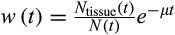, where gives the numbers of terminally differentiated cells at age , is the total number of cells ( ), and the last term is the probability that the organism has escaped extrinsic mortality up to age .

To find and the times of maturity and death, we need to describe how the ontogenetic strategy spreads new cells into the state space. We assume that an organism grows towards the maturity threshold before it has reached this size, and aims to maintain the number of terminally differentiated cells thereafter (which requires compensating for cells that have died either because of a baseline cell turnover , see below, or because of being killed as part of the ontogenetic strategy). Thus, both before maturity and afterwards, the organism begins a time step by measuring the difference between the target number of terminally differentiated cells ( ) and its current number ( ). The deficit is then defined as 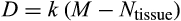, rounded up to the nearest integer, where the multiplication with a constant makes growth before maturity approximate a von Bertalanffy trajectory (Karkach, 2006).

In case of a positive deficit, up to stemlike cells will divide. If , the number of dividing cells is , which makes the deficit vanish. If , then all cells divide, and the deficit diminishes. In both cases, will be calculated a new in the next time step. If there is an excess of stemlike cells to choose from (the first case), the precise identity of cells chosen for division follows component of the organism's ontogenetic strategy, in the following manner.

Stemlike cells occur in different states of differentiation 0, 1,…, T−1. Ontogenetic strategy component is defined as the relative division propensity of a given level of differentiation compared with the previous one ( 1 means that propensities increase with level of differentiation). Cells are chosen (without replacement) to divide with relative propensities that are proportional to , where is the cell's current degree of differentiation, until the appropriate (see above) number of cells has been chosen. A cell's position along the or axis does not directly impact its likelihood of becoming a dividing cell, though patterns of covariation are likely to arise because cells far on their path to full differentiation are also likely to have progressed further from the 0 state along these axes too. Thus, if is high, divisions use stem cells sparingly, which also means that divisions occur more commonly in cells that have already incurred some damage.

Once the state-specific numbers of dividing cells are known, each division is performed taking into account strategy components and (Figure 1c). We assume that differentiation only occurs during cell divisions. The division occurs asymmetrically with probability , in which case one daughter cell is placed into the soma one step further along the differentiation axis while the other daughter cell does not change in its level of differentiation (for placements along the other axes, see below). With probability 1 , the cell divides symmetrically, and in this case, component of the strategy is also relevant. Each of the two daughter cells enters the soma as either one step more differentiated than the parent (with probability , applied independently for both daughters) or at the same level of differentiation as the parent (with probability 1 , interpretable as replenishment of the pool of stemlike cells). Thus, as a whole, with probability (1 ) a division occurs symmetrically and yields in two daughter cells that are both more differentiated than their parent, whereas with probability (1 ) (1 ) it yields in two cells at the identical level of differentiation as the mother cell, and finally, with probability the division produces one daughter that is more differentiated than the parent and another daughter that remains at the original differentiation level.

After each cell division, we also need to specify the positions of the new daughter cells along the and axes. Since the axis tracks the number of cell divisions, the new location along this axis is always one step further than the old location (and since only stemlike cells, up to H−1, can be chosen to divide). Mutations that increase DNA damage occur only during cell divisions. Regarding DNA damage, each new daughter cell can be at the same location along the axis (with probability 1 ) or with an increased level of DNA damage, that is one step further along the axis (probability ).

At the end of a division round, we apply various sources of mortality to cells (Figure 1d). Parental cells have at this point become two daughter cells, necessitating removing the original parent from the soma. Cells that have reached the Hayflick limit (state ) are also removed. Furthermore, the ontogenetic strategy has two components, and , that aim to remove damaged cells (cells that are far along the axis regardless of their position along other axes), but we assume that the recognition of damage is imperfect. A proportion of cells with are killed, where is a cell's true location along the axis and an error term reflects the difficulty of determining precisely how damaged a cell is. Since recognized damage is a real number (not restricted to integer values), we also allow A to take real number values. The organism cannot evolve a smaller , but it can evolve a suitable , with a clear trade-off: a low is good for reliable removal of all damage, but a large number of healthy cells will then be removed too, depleting the pool of stemlike cells potentially too quickly. Finally, any of the cells that survive the above mortality risks die with probability , reflecting baseline cellular mortality (cell turnover), applied independently to each cell.

3 RESULTS

Optimized life histories reached much higher lifetime fitness at small than at large body sizes (Figure 2a). While surprising at first sight, note that our model did not give large organisms any of the advantages often associated with body size (Kingsolver & Pfennig, 2004). We therefore do not examine selection to become large per se, but ask how organisms deal with the increased difficulties that creating a larger body entails. A major challenge is that reaching maturation size takes more time if the required size is larger (Figure 2b). Meeting this challenge requires changing some, but not all, components of the ontogenetic strategy in a systematic manner. The probability of differentiation ( ) declines with body size (Figure 2d), while the number of levels to terminal differentiation ( ) increases (Figure 2e). Also, at larger body sizes, the damage response threshold ( ) was never found to be low, whereas low body sizes can be viable with a range of values for (Figure 2h).

The remaining four traits ( , , and ; Figure 2c,f,g, and i, respectively) did not show as clear patterns related to body size. There are two potential explanations: that the fitness landscape is very flat with respect to these traits, or that the traits matter for fitness, but occur in the form of coadapted gene complexes (Schwander, Libbrecht, & Keller, 2014; Sinervo & Svensson, 2002). In the latter case, an overall “shotgun-like” pattern (Figure 2c, f, g, and i) has more structure than is apparent at first sight: a rugged multidimensional fitness landscape may produce high fitness at particular combinations of trait values, rather than peaking at a single value for each trait independently of the six other traits. For example, the lower values of in Figure 2d associate with the higher in Figure 2c. When symmetric divisions contribute less to tissue differentiation (a low ), an organism might not suffer if it resorts to more asymmetric divisions (a high ); at lower , will matter more (Figure S1). We tested for the ruggedness of the landscape by using the outcomes of optimizing the ontogenetic strategy four times independently (from different starting points). In case of coevolved gene complexes, creating a new strategy by changing one of the seven evolved components to the outcome of a parallel optimization (for the same body size) should reduce fitness, which we found to be the case (Appendix S1).

We next ask whether evolved ontogenetic strategies form constraints for evolving a different body size: can a strategy that evolved at a small body size reach high fitness if implemented in a life history with a larger maturation size; and is the reverse true (from large to small body sizes)? Smaller organisms might fail to operate for long enough if growth to become large (which takes time) is now required. Reciprocally, strategies evolved in larger organisms might be expected to fail if their slow way of forming tissues (low , and many levels to full differentiation, ) means that they are not “ready” when maturing at small size. We found clear evidence for the first type of failure (from small to large) but not the second (Figure 3); strategies evolved in larger organisms were relatively robust to changes in body size, allowing organisms of the entire tested size range to grow to maturation. Interestingly, the independent parallel optimizations for the “evolved while small” strategies varied in the range of size increases that they tolerated (for particularly clear cases see Figure 3b). Thus, while performing equivalently when small, some coadapted combinations permit size increases much better than others.

The causes of death were different across the examined body sizes. Optimized strategies (Figure 4a) typically manage the soma well enough so that no other causes of death than extrinsic mortality occur until very few individuals are alive (due to extrinsic mortality). In the rare cases where an optimized strategy dies from other causes, then the cause relates to running out of stem cells at small body sizes, and to cancer at large body sizes. However, if a small organism attempts to grow larger (than during its evolutionary past that optimized its ontogenetic strategy), the failures typically relate to running out of stem cells (Figure 4b,c), supporting the interpretation that small organisms do not need as sophisticated management of the stem cell pool as large ones. Large organisms that turn small perform well because the now diminished number of cell divisions protect against cancer, and simultaneously, their stem cells do not run out as they were already well managed; extrinsic mortality then remains the virtually only cause of death (left part of Figure 4d).

4 DISCUSSION

Our model integrates seven different aspects of ontogeny (tissue differentiation in the presence of cancer risk) into a single model, to ask (a) how organisms are expected to manage their stem (and stemlike) cell populations during tissue differentiation while also avoiding cancer, and (b) whether the evolved strategies need to be modified in case organisms change their body size over evolutionary time.

Regarding our first question, it appears that some aspects of division and differentiation strategies are under stronger selection than others, with the fitness landscape as a whole showing signs of ruggedness: for a given body size, different initial trait combinations led to different solutions to the same problem while reaching overall similar fitness. This suggests that organisms of similar size and lifespan, and hence with comparable cell-management requirements, can grow and survive using a diversity of mechanisms. Since cancer was only one of several ways to die in our model, our results also highlight the potential for similar ruggedness in stem cell pool replenishment strategies: there are many ways to succeed in keeping the stemlike cell population large enough for long enough, such that the remaining challenges relate to extrinsic mortality only (we here follow a modelling tradition of calling age-independent mortalities that the organism cannot change as “extrinsic”; Abrams, 1993; Boddy et al., 2015; Carnes & Olshansky, 1997). These could potentially explain the variation in telomere length or telomerase expression in mammals, especially in smaller ones (Gomes et al., 2011). While not explicitly modelled by us, it is intriguing that naked mole rats and blind mole rats might be using a common adaptation (secretion of high molecular mass hyaluronan, HMM-HA) that evolved independently for their ecological conditions (living underground) to counteract cancer risk via different pathways (Seluanov, Gladyshev, Vijg, & Gorbunova, 2018). Finally, from a molecular point of view, how the traits that make part of an ontogenetic management strategy evolve might also depend on more interactions between genes than we modelled, adding to our view of rugged landscapes: here, we assumed no interactions between genes via regulatory networks (Trigos, Pearson, Papenfuss, & Goode, 2019), but these could change which pathways are “available” to an organism.

Turning to our second question, the body size dependence of the ontogenetic strategy, we found clear evidence that the strategy requires modification when mature body size changes. However, this finding comes with two subtleties. Firstly, not all components of the strategy showed strong relationships with body size. However, the coadaptedness of strategy components has consequences for the strategies' robustness when tested in the context of a novel body size. Specifically, forcing two (or more) independently derived strategies to perform at a novel (larger) body size revealed differences in the range of body sizes that a strategy can still cope with. When a strategy failed when tested in a larger body, the problems related to running out of stem cells rather than cancer. This is interesting in the context of Peto's paradox (Caulin & Maley, 2011; Peto et al., 1975), which is expressible as “all else being equal, more cell divisions should lead to a higher cancer risk.” In our model, small organisms died due to stem cell depletion if they became large without being given an opportunity to adapt their ontogeny to their new life history. The cancer risk reappeared only when they used “large”-adapted ontogenetic strategies.

Secondly, there was an interesting asymmetry: large organisms, which adapted to their larger size by having a smaller per-cell probability of differentiation, a not too eagerly applied threshold of killing damaged cells, and many differentiation steps before a tissue is formed, possessed ontogenetic strategies that also worked well when tested in small organisms. Although computational limitations prevented us from scaling our study up to cell numbers involved in large metazoans, we see no reason why such asymmetries would not continue playing a role at such sizes. Our finding is therefore interesting in the context of macroevolutionary changes in body sizes, where it is known that miniaturization, when it happens, appears to proceed much faster than the (as a whole more common; Kingsolver & Pfennig, 2004) increase in body size over evolutionary time (Evans et al., 2012). It also fits well with findings of intraspecific variation in humans, where size increases associate with heightened cancer risk (Green et al., 2011; Nunney, 2018), while hereditary forms of dwarfism, at least in the context of the so-called Laron syndrome, appear to offer cancer protection (Laron, Kauli, Lapkina, & Werner, 2017).

Note that our model should be complemented with additional considerations when making predictions about rates of evolution. Eco-evolutionary dynamics has features that we did not take into account: larger organisms tend to have smaller effective population sizes (with population density as a proxy; Damuth, 1981), which can slow down the rate of adaptive evolution (Lanfear, Kokko, & Eyre-Walker, 2014). We sidestepped such issues as we simply re-simulated optimized ontogenies for novel body sizes, rather than taking existing ontogenies as starting points (while beyond the scope of the current paper, we will examine the consequent phylogenetic inertia in our future work). Generation times also vary with body size (Martin & Palumbi, 1993); our model is an “all else being equal” investigation of body size, where time to maturity takes longer for larger maturation sizes, but, for example, extrinsic mortality does not change. It is interesting to note that our choice to have very few differences between ancestral and novel conditions (no ecological change apart from time it takes to mature, which emerges naturally in the model) still led to a prediction that parallel runs of the optimization procedure will differ in how easily a small-bodied organism can evolve a larger size. Some ontogenetic strategies collapsed to zero fitness at much smaller demands to become big, than others. We interpret this finding as a prediction that some fortuitous small multicellular organisms have preadaptations to grow over macroevolutionary time, while others face stronger intrinsic constraints. This adds ontogenetic challenges to the reasons why Cope's rule, the increase in body sizes in macroevolutionary lineages (Clauset & Erwin, 2008; Stanley, 1973), is expected to be a rather stochastic “rule” (see, e.g., Heim, Knope, Schaal, Wang, & Payne, 2015; Liow & Taylor, 2019).

Some of our findings are, at least at first sight, unexpected. The damage response threshold reflects how many mutations are tolerated before a cell is recognized as damaged and killed (e.g. via apoptosis, or by other cells; we do not specify the exact mechanism) with probability . Based on an important study on elephant cells responding more readily to damage than human cells (Abegglen et al., 2015), one might expect to decrease and to increase with body size, but such responses did not emerge in our model. Instead, small organisms could function across a wide range of values for both and , while larger somas were never found to be built with small values of . This apparent mismatch between Abegglen et al., (2015) and our results disappears, however, when taking into account coadaptation between different ontogenetic strategy components. Large organisms also evolved to use more steps ( ) to full differentiation, which also gives cell lineages more cumulative opportunities (in the form of a higher number of divisions) to accumulate damage. A higher , when it also associates with a higher , therefore does not necessarily mean that fewer cells are observed to be killed in any phenotype. When is high, cells have more opportunities to reach a category of damage that sees them killed. Moreover, since running out of stemlike cells was a real threat in our model, it appears that this penalizes against very strict “quality control” of cells; no strategy can succeed if sufficient cell numbers are not maintained, while cancer can at least probabilistically be avoided (under a multistep model of oncogenesis; Armitage & Doll, 1954; Calabrese & Shibata, 2010; Nunney, 1999). These considerations add to our general message that there are many complementary ways to create a soma of a certain body size.