Point-optimal panel unit root tests with serially correlated errors
Summary
Generalizations of the point-optimal panel unit root tests of Moon, Perron and Phillips (MPP) are developed to cover cases of serially correlated errors. The resulting statistics involve two modifications relative to those of MPP: (a) the error variance is replaced by the long-run variance; (b) centring of the statistic is adjusted to correct for second-order bias effects induced by the correlation between the error and lagged dependent variable.
1. Introduction
 and an (unobserved) stochastic component
  for some observable panel observations
  for individual
  in period
  satisfying
 (1.1)
(1.1) is an error term that has zero mean and is stationary over time, and
  for simplicity. Dynamic panel models with incidental trend components of this type arise in many applications in microeconometrics, multicountry growth studies and international finance. Empirical interest often centres on the individual dynamics and on whether there is commonality and persistence across individuals (i.e. that the autoregressive parameters
  are all unity) or whether such commonality occurs for certain subgroups of individuals.
 (1.2)
(1.2) is a sequence of i.i.d. random variables and κ is a parameter defining the width of the vicinity as
  . The null hypothesis of interest is then
 (1.3)
(1.3) (1.4)
(1.4)The MPP tests are point optimal in the sense of giving highest power against a specific set of  . These tests were derived under the assumption that the error term
  is independent across individual units and over time. They represent a panel extension of the work of Elliott et al. (1996) in the time-series case where the autoregressive parameter converges to unity at a rate of
  , regardless of the deterministic component in the model.
Independence assumptions are not realistic in many empirical applications and in this work we extend the MPP tests by allowing for serially correlated errors  . In their Section 6.4 (p. 436), MPP briefly mentioned this extension. Here, we provide explicit test statistics that have optimal asymptotic properties. The modified tests replace estimated variances of the errors in MPP with estimated long-run variances, and adjust centring terms. Our main purpose is to provide the form of the modified tests and to give their asymptotic properties so that they can be used in empirical work.
The paper is organized as follows. In Section 2., we show how to construct the tests, give results for cases with no fixed effects, fixed effects and incidental trends, and discuss implementation. In Section 3., we report some simulation findings. We conclude in Section 4, and in the Appendix we provide technical derivations and supporting lemmata.
2. Tests under Serial Correlation
Following MPP, in the following analysis, we consider three deterministic trend cases: (a) no individual effects (i.e.  and
and  ); (b) fixed effects (i.e.
  ); (c) heterogeneous or incidental linear trends (i.e.
  ). In each case, we proceed in three steps. First, we define the likelihood ratio (
 ) statistic under Gaussianity, which is known to be optimal by the Neyman–Pearson lemma when the null and alternative hypotheses are simple. Then, we show that this statistic can be approximated by a simpler version with parameters that are consistently estimable. Finally, we derive the asymptotic distribution of this approximation (with appropriate recentring). In all three cases, this asymptotic distribution coincides with the one in MPP.
 and U the
  observation matrices whose
  th elements are
  ,
,  ,
,  ,
,  and
and  , respectively. Define the
  vectors
  ,
,  and set
  , where
  . Define
  ,
,  and
and  , where
  . Let
. Let  ,
,  ,
,  and
and  denote the transpose of the ith row of Z, Y,
  and U, respectively. With this notation, the model has the matrix form

 .
.Define  ,
,  and
and  as the variance of
  , the long-run variance of
  and the one-sided long-run variance of
  , respectively, so that
  . Let Σ, Ω and Λ be the diagonal matrices with elements
  ,
,  and
and  , respectively. Define
  as the
  covariance matrix of
  and
and  as the
  covariance matrix of
  . As in MPP, we assume that the errors
  are cross-section independent over i.
 in the local alternative 1.2 is a sequence of i.i.d. random variables with bounded support.1 Let
  ,
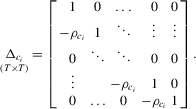
,  and define the quasi-difference operator
 and
and  .
.
Throughout the paper, we assume panel linear process errors with conditions similar to those in the literature (e.g. Phillips and Moon, 1999). Let  , let
, let  be the spectral density of
  , and let
  .
.
Assumption 2.1.(a)  , where
  with
with  and
and  for some
  ; (b)
; (b)  for some
  ,
,  ,
,  ,
,  ; (c)
; (c)  and for
  and some constant M.
These conditions extend the serial dependence restrictions of Elliott et al. (1996) (e.g. their Condition A) to heterogeneous panels. Assumption 2.1(a) assumes that the error term  follows a linear process that is heterogeneous across i. The higher moments are needed to ensure the large
  asymptotics of panel data that are heterogeneous across i and serially correlated over t. Under cross-sectional homoscedasticity, these moment conditions could be weakened. Assumptions 2.1(b) and 2.1(c) restrict the temporal dependence of the error term
  to be ‘weak’ uniformly across i. These restrictions exclude long memory type strong dependence. The conditions in Assumption 2.1 are quite weak and are satisfied by many parametric weak dependent processes, such as stationary and invertible ARMA processes.
While Assumption 2.1 is quite general in terms of the serial correlation that is allowed, it is restrictive in that it assumes that all cross-sectional units are independent. This assumption is not reasonable for many interesting empirical data sets, such as cross-country studies where business-cycle effects are likely to induce correlation across countries. As in MPP, we conjecture that the procedures proposed below are valid after appropriate orthogonalization is applied, for example, after the removal of common factors as in Moon and Perron (2004), Bai and Ng (2004) or Phillips and Sul (2003). Moreover, the development of optimal procedures under cross-sectional dependence is beyond the scope of the current paper.
2.1. No fixed effect: 
 , the model becomes

 , so that the rate coefficient
  , and one-sided alternatives in which the support of
  is a bounded interval
  for some
  so that
  under this alternative. In terms of the first moment of
  , the hypotheses about
  are
are
 (2.1)
(2.1) (2.2)
(2.2) are Gaussian so that
  with known
  and the initial conditions
  are all zeros.2 By the Neyman–Pearson lemma, rejecting a small value of the log-likelihood ratio test statistic
 (2.3)
(2.3) for
for  against the simple alternative
  for
for  . When the alternative is 1.4 with 2.2, this becomes a point-optimal test.
In order to implement the optimal test statistic 2.3, we need an estimate of the entire  covariance matrix
  . This is a huge high-dimensional covariance estimation problem in a non-parametric set-up. The following theorem provides an approximation of the likelihood ratio test statistic in 2.3 with a statistic where the unknown nuisance parameters are consistently estimable.
Theorem 2.1.Let Assumption 2.1 hold with  . Assume that
  → 0 as
  . Then, for
  , we have

 (2.4)
(2.4) with an adjustment of the one-sided long run variance
  . The one-sided long-run drift correction appears to be a result of the correlation between the stationary error
  and the lagged dependent variable
  . The main advantage of this formulation is that it involves quantities (Ω and Λ) that can be estimated consistently.
 is the sum vector and
  .
.
Remark 2.1.We can interpret the test statistic  as an asymptotic version of the point-optimal test for panel unit roots with possible serial correlation of unknown form in the error term.
Remark 2.2.Compared to the corresponding statistic in MPP, which makes no allowance for serial correlation, there are two differences in  . First, as discussed in MPP, we use the long-run covariance matrix
  instead of the variance matrix
  as the weight matrix. In addition, we recentre the statistic by subtracting the term
  , which corrects for the correlation between the stationary error
  and the lagged dependent variable
  . This term is not required for the test under temporal independence.
Remark 2.3.The limit distribution of  is the same limit as in MPP (see their Theorem 6).
2.2. Time-invariant fixed effects: 
 are fixed over time. This corresponds to the standard fixed effects model. In this case, the model has matrix form

 with known
  and the initial conditions
  are all zeros. Then, rejecting a small value of the test statistic,
 (2.5)
(2.5) for
for  and the alternative
  for
for  is known as the uniformly most powerful invariant test that is invariant with respect to the transformation
  for arbitrary
  . Against the alternative in 1.4, this becomes a point-optimal invariant test (e.g. Dufour and King, 1991).
As mentioned in the previous section, this statistic is difficult to implement because of the presence of  , the full
  covariance matrix of the error. This again motivates the use of an approximation.
Theorem 2.3.Let Assumption 2.1 hold with  and let
  as
as  . Then, for
  , we have

Remark 2.4.This approximation is derived under the stronger rate condition  → 0 as
  in place of the condition
  as
as  that is used without fixed effects.
Remark 2.5.The approximation involves the same correction for second-order bias as in the case without fixed effects.

Theorem 2.4.Let Assumption 2.1 hold and let  as
as  . Then, under the local alternative
  , we have

 .
.
This asymptotic distribution is the same as without fixed effects and as in MPP (see their Theorem 9).
2.3. Incidental trends: 
Under heterogeneous linear trends, we follow MPP and use local neighbourhoods of unity that shrink at the slower rate of  , so that the rate coefficient is
  . The alternative might be two-sided; that is,
  with mean
  and variance
  , with a support that is a subset of a bounded interval
  , where
  ,
,  . The slower rate of shrinkage in the local neighbourhoods of unity is the result of the presence of heterogeneous trend effects in the panel. The presence of these incidental trends reduces discriminatory power in testing for the presence of common stochastic trends, so wider localizing intervals are needed to attain non-trivial power functions.
 with known
  and the initial conditions
  are all zeros. Then, similar to the case of time-invariant fixed effects, rejecting a small value of the test statistic,

 for
for  and the alternative
  for
for  , is known as the uniformly most powerful invariant test (with respect to the linear transformation
  for arbitrary
  ), and against the alternative in 1.4, it becomes a point-optimal invariant test. As before, we start by proving the validity of an approximation to this log-likelihood ratio.
Theorem 2.5.Let Assumption 2.1 hold with  and let
  as
as  . Then, for
  , we have

Remark 2.6.This approximation is derived under the condition  as
as  , which is a stronger rate condition than that used for the intercepts case.
Remark 2.7.As before, the correction is a result of the presence of a second-order bias term arising from the correlation between the lagged dependent variables and the error term.


Theorem 2.6.Let Assumption 2.1 hold and let  as
as  . Then, under the local alternative
  , we have

As before,  reduces to the statistic from MPP when there is no serial correlation, and it has the same asymptotic distribution as in Theorem 13 of MPP.
2.4. Implementation of the tests
The test statistics  ,
,  and
and  depend on unknown parameters
  ,
,  and
and  . Let
. Let  ,
,  and
and  be consistent estimators of
  ,
,  and
and  , respectively. Similarly define the diagonal matrices of these elements as
  ,
,  and
and  . To implement these tests, we can replace Σ, Ω and Λ in
  ,
,  and
and  with
with 
 and
and  and we denote the test statistics as
  ,
,  and
and  . We assume the following regarding these estimators.
Assumption 2.2.Under the local alternative,  ,
,  and
and  .
.
Remark 2.8.An example of  that satisfies Assumption 2.2 is the time-series sample variance of

Remark 2.9.When kernel spectral density estimation is used for  and
and  with bandwidth h, Assumption 2.2 is satisfied if: (a) the kernel function
  is continuous at zero and all but a finite number of other points, satisfying

 and
and  for some
  where parameter m is defined in Assumption 2.1(b); (b) the bandwidth h satisfies
 (2.8)
(2.8) and
and  ; see, e.g., Moon and Perron (2004). If
  for some
  and
and  , then the bandwidth condition 2.8 is satisfied if


 . MPP have shown that the optimal choice of
  is
is  . With this choice, the likelihood ratio statistics above attain the power envelope. However, this choice is infeasible because
  are the parameters under test. MPP proposed the assumption of a common
  for all cross-sectional units, and they called this test a common point-optimal (CPO) test. With this choice,
  , and we can deduce from Theorems 2.2, 2.4 and 2.6 that under the null hypothesis,
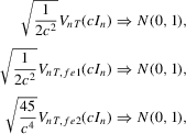

The surprising result here is that neither distribution depends on the choice of c used to construct the test. This feature implies that the power is the same for all choices of c asymptotically, although that choice matters in finite samples. Based on the simulation evidence provided in MPP, we set  in the simulation below. Of course, this choice of
  is not optimal unless the alternative hypothesis is homogeneous (
 for all i) and results in a power loss relative to the power envelope.
3. Monte Carlo simulations


 ), positive AR (
 and
and  ), negative AR (
 and
and  ), positive MA (
 and
and  ) and negative MA (
 and
and  ).
).In all cases, we allow for heterogeneity and draw the idiosyncratic variance  from a uniform distribution,
  . This variance is scaled such that the scale of
  is the same for all cases. In both the incidental intercepts case
  and the incidental trends case
  , the parameters are drawn from
  .
.
We focus the study on the size and size-adjusted power of the CPO test with  for all i, because MPP advocated that choice. For size calculations, we set
  for all i, which corresponds to
  for all i in our local-to-unity framework. For power, we draw
  from a uniform distribution between 0 and 8, as in one of the experiments of MPP. This specification ensures that power should be roughly constant as N and T increase.
We draw comparisons with two existing tests, those of Levin et al. (2002), hereafter LLC, and Im et al. (2003), hereafter IPS. We take three values for n (10, 25 and 100) and two values of T (100 and 250). All tests are conducted at the 5% significance level, and the number of replications is set at 2,000.
Estimation of the long-run variance and one-sided long-run variance is critical to the performance of the CPO test. We estimate these quantities in two ways based on demeaned first differences, as in Remark 2.8. The first method is a non-parametric estimator with quadratic spectral kernel and bandwidth selected in a data-based manner using the Andrews (1991) rule with no pre-whitening (PW). The second method uses pre-whitening where the appropriate model is chosen using BIC among the AR(1), MA(1), ARMA(1,1) and constant-only models. In the case of the LLC test, we follow the recommendation of Levin et al. (2002) and use a Bartlett kernel with a bandwidth equal to  . Westerlund (2009) has shown that this choice gives the LLC test higher power than selecting the bandwidth in a data-dependent way. Similarly, for the IPS and LLC tests, the choice of lag augmentation is critical for performance. We choose this in a data-dependent way by BIC with a maximum of six lags. For both of these tests, we use the finite-sample adjustments provided in the original papers.
The size results are reported in Tables 1 and 3 for the incidental intercepts and trends cases respectively, while size-adjusted power is in Tables 2 and 4. For each of the five serial correlation specifications, each row corresponds to a different test.
 |
 |
 |
||||||||
 |
 |
 |
||||||||
| 100 | 250 | 500 | 100 | 250 | 500 | 100 | 250 | 500 | ||
|---|---|---|---|---|---|---|---|---|---|---|
| White noise | This paper, no PW | 1.6 | 2.2 | 2.6 | 2.8 | 3.2 | 3.6 | 4.2 | 3.7 | 5.2 |
| This paper, PW | 2.4 | 2.4 | 2.5 | 3.0 | 3.8 | 4.5 | 0.6 | 2.5 | 4.4 | |
 |
MPP (2007) | 2.9 | 2.4 | 2.5 | 4.8 | 3.7 | 4.4 | 4.3 | 3.6 | 4.7 |
 |
IPS | 6.4 | 3.7 | 4.9 | 7.0 | 5.2 | 5.2 | 8.4 | 6.9 | 5.1 |
| LLC | 5.8 | 4.4 | 4.1 | 5.8 | 5.3 | 3.4 | 6.0 | 5.0 | 3.5 | |
| Positive AR | This paper, no PW | 1.7 | 1.8 | 2.9 | 2.4 | 2.8 | 3.3 | 4.5 | 4.5 | 4.9 |
| This paper, PW | 2.3 | 2.1 | 3.0 | 1.7 | 2.3 | 3.0 | 0.7 | 0.4 | 2.4 | |
 |
MPP (2007) | 0.3 | 0.5 | 0.8 | 0.1 | 0.1 | 0.1 | 0.0 | 0.0 | 0.0 |
 |
IPS | 5.0 | 4.4 | 3.6 | 4.7 | 3.9 | 3.5 | 3.1 | 3.1 | 3.5 |
| LLC | 5.0 | 4.2 | 4.0 | 4.3 | 4.3 | 3.7 | 2.6 | 2.8 | 3.9 | |
| Negative AR | This paper, no PW | 1.7 | 2.1 | 2.2 | 2.5 | 3.2 | 4.0 | 5.4 | 4.2 | 5.2 |
| This paper, PW | 2.0 | 2.5 | 2.1 | 1.2 | 2.6 | 3.3 | 0.3 | 1.5 | 2.2 | |
 |
MPP (2007) | 12.7 | 13.2 | 13.6 | 30.7 | 30.3 | 32.4 | 82.2 | 81.6 | 83.9 |
 |
IPS | 12.8 | 7.3 | 5.4 | 20.4 | 9.4 | 7.2 | 42.6 | 15.3 | 9.3 |
| LLC | 9.0 | 5.8 | 4.2 | 12.0 | 7.0 | 4.0 | 20.8 | 8.5 | 4.3 | |
| Positive MA | This paper, no PW | 1.4 | 1.7 | 2.6 | 2.1 | 3.0 | 3.7 | 4.3 | 4.5 | 4.8 |
| This paper, PW | 2.5 | 2.6 | 3.0 | 2.7 | 3.2 | 4.1 | 1.6 | 3.5 | 4.5 | |
 |
MPP (2007) | 0.7 | 0.7 | 0.6 | 0.3 | 0.2 | 0.6 | 0.0 | 0.0 | 0.0 |
 |
IPS | 6.6 | 6.1 | 5.7 | 6.8 | 6.4 | 6.0 | 7.1 | 7.4 | 8.4 |
| LLC | 6.1 | 5.9 | 4.7 | 5.4 | 6.0 | 4.6 | 5.2 | 7.2 | 5.6 | |
| Negative MA | This paper, no PW | 1.3 | 2.0 | 2.6 | 2.3 | 3.5 | 3.6 | 4.6 | 4.5 | 4.3 |
| This paper, PW | 1.5 | 2.4 | 3.0 | 0.9 | 3.1 | 4.0 | 0.0 | 1.6 | 3.5 | |
 |
MPP (2007) | 17.0 | 16.7 | 17.6 | 40.7 | 44.1 | 40.7 | 93.0 | 91.8 | 93.1 |
 |
IPS | 25.0 | 13.8 | 10.2 | 40.4 | 22.6 | 14.3 | 85.0 | 50.0 | 32.9 |
| LLC | 15.6 | 9.4 | 6.9 | 22.2 | 12.3 | 6.5 | 56.6 | 25.9 | 14.4 | |
Note
- The table reports the rejection frequency (in %) of a 5% test for a panel unit root. “This paper, no PW” refers to the common point optimal (CPO) tests proposed in this paper with no pre-whitening used when estimating long-run variances and c = 1. “This paper, PW” refers to the CPO tests in this paper with pre-whitening when estimating long-run variances. “MPP (2007)” refers to the CPO tests with c = 1 in MPP that do not allow for serial correlation. “IPS” is the t-bar test of Im et al. (2003) and “LLC” is the test of Levin et al. (2002).
 |
 |
 |
||||||||
 |
 |
 |
||||||||
| 100 | 250 | 500 | 100 | 250 | 500 | 100 | 250 | 500 | ||
|---|---|---|---|---|---|---|---|---|---|---|
| White noise | This paper, no PW | 41.6 | 49.3 | 52.9 | 53.0 | 62.6 | 62.8 | 66.4 | 75.2 | 71.7 |
| This paper, PW | 43.2 | 54.8 | 52.5 | 45.1 | 62.2 | 62.6 | 40.5 | 73.0 | 73.4 | |
 |
MPP (2007) | 50.5 | 55.1 | 54.1 | 59.4 | 66.4 | 62.5 | 76.7 | 78.7 | 74.6 |
 |
IPS | 13.2 | 18.1 | 12.9 | 16.8 | 17.5 | 16.9 | 21.6 | 18.6 | 21.3 |
| LLC | 3.7 | 1.9 | 1.1 | 5.3 | 3.3 | 2.8 | 5.7 | 3.8 | 3.1 | |
| Positive AR | This paper, no PW | 42.9 | 51.8 | 45.3 | 54.8 | 62.8 | 63.6 | 63.7 | 69.5 | 73.4 |
| This paper, PW | 48.8 | 53.1 | 48.0 | 59.5 | 64.1 | 62.2 | 63.5 | 73.5 | 74.8 | |
 |
MPP (2007) | 52.0 | 54.5 | 45.4 | 62.4 | 60.7 | 63.9 | 72.2 | 73.1 | 73.7 |
 |
IPS | 12.0 | 13.0 | 16.1 | 12.4 | 17.2 | 14.8 | 21.3 | 19.5 | 20.7 |
| LLC | 3.1 | 2.3 | 1.8 | 3.5 | 2.7 | 1.6 | 6.0 | 5.2 | 3.5 | |
| Negative AR | This paper, no PW | 42.8 | 48.3 | 51.3 | 53.2 | 60.3 | 61.1 | 63.3 | 72.0 | 72.4 |
| This paper, PW | 45.0 | 52.5 | 51.4 | 47.2 | 59.8 | 61.0 | 40.0 | 69.6 | 76.3 | |
 |
MPP (2007) | 48.4 | 47.8 | 50.5 | 62.9 | 59.6 | 60.6 | 70.1 | 71.5 | 74.7 |
 |
IPS | 13.0 | 14.6 | 14.4 | 19.7 | 16.1 | 15.8 | 22.0 | 20.0 | 19.0 |
| LLC | 5.2 | 2.6 | 1.3 | 6.1 | 2.3 | 2.4 | 7.9 | 4.6 | 3.2 | |
| Positive MA | This paper, no PW | 44.2 | 48.0 | 51.3 | 52.8 | 63.2 | 59.8 | 63.6 | 72.8 | 73.0 |
| This paper, PW | 47.6 | 51.8 | 53.5 | 59.0 | 64.5 | 61.2 | 58.4 | 74.7 | 74.8 | |
 |
MPP (2007) | 52.2 | 54.0 | 50.9 | 61.3 | 66.4 | 64.2 | 72.3 | 75.8 | 75.2 |
 |
IPS | 10.4 | 12.7 | 12.1 | 14.3 | 16.4 | 17.4 | 17.9 | 20.8 | 18.7 |
| LLC | 2.6 | 1.9 | 1.1 | 4.6 | 2.7 | 1.9 | 5.5 | 4.0 | 3.4 | |
| Negative MA | This paper, no PW | 41.4 | 49.4 | 47.5 | 54.8 | 55.5 | 59.9 | 65.9 | 72.7 | 77.9 |
| This paper, PW | 46.7 | 51.8 | 48.7 | 43.0 | 57.6 | 62.2 | 32.6 | 68.1 | 77.8 | |
 |
MPP (2007) | 48.6 | 48.7 | 46.3 | 57.9 | 57.2 | 58.4 | 68.8 | 70.0 | 72.1 |
 |
IPS | 15.0 | 16.7 | 14.2 | 21.2 | 15.3 | 18.8 | 23.9 | 26.7 | 22.5 |
| LLC | 8.1 | 2.6 | 1.6 | 8.5 | 4.3 | 3.7 | 11.8 | 6.7 | 3.6 | |
 |
 |
 |
||||||||
 |
 |
 |
||||||||
| 100 | 250 | 500 | 100 | 250 | 500 | 100 | 250 | 500 | ||
|---|---|---|---|---|---|---|---|---|---|---|
| White noise | This paper, no PW | 0.0 | 0.1 | 0.5 | 0.0 | 0.6 | 1.5 | 0.0 | 0.5 | 0.9 |
| This paper, PW | 1.0 | 1.0 | 1.4 | 1.8 | 2.3 | 2.7 | 1.4 | 4.1 | 4.5 | |
 |
MPP (2007) | 1.7 | 1.3 | 1.4 | 4.6 | 2.5 | 2.9 | 7.2 | 5.1 | 4.4 |
 |
IPS | 8.2 | 5.5 | 5.2 | 10.6 | 5.6 | 4.4 | 14.9 | 7.5 | 6.4 |
| LLC | 6.4 | 4.5 | 2.1 | 5.8 | 4.3 | 1.1 | 4.8 | 4.4 | 0.5 | |
| Positive AR | This paper, no PW | 0.0 | 0.0 | 0.5 | 0.0 | 0.4 | 1.5 | 0.0 | 0.2 | 1.2 |
| This paper, PW | 0.8 | 0.4 | 1.0 | 1.6 | 2.2 | 2.2 | 2.1 | 2.1 | 2.0 | |
 |
MPP (2007) | 0.0 | 0.0 | 0.1 | 0.0 | 0.0 | 0.0 | 0.0 | 0.0 | 0.0 |
 |
IPS | 5.3 | 3.5 | 4.4 | 4.2 | 3.0 | 4.0 | 3.8 | 2.8 | 3.3 |
| LLC | 3.7 | 2.7 | 1.7 | 2.0 | 2.6 | 0.9 | 0.7 | 1.2 | 0.2 | |
| Negative AR | This paper, no PW | 0.0 | 0.1 | 0.5 | 0.0 | 0.2 | 1.0 | 0.0 | 0.3 | 1.3 |
| This paper, PW | 0.4 | 0.6 | 0.7 | 0.5 | 1.2 | 1.9 | 0.2 | 1.7 | 2.1 | |
 |
MPP (2007) | 22.2 | 19.8 | 20.3 | 61.7 | 58.4 | 56.8 | 99.3 | 99.3 | 99.1 |
 |
IPS | 25.3 | 10.7 | 7.1 | 40.6 | 15.6 | 8.9 | 84.1 | 31.7 | 13.7 |
| LLC | 16.9 | 7.6 | 2.8 | 24.5 | 9.4 | 1.6 | 53.8 | 14.5 | 0.5 | |
| Positive MA | This paper, no PW | 0.0 | 0.2 | 0.5 | 0.0 | 0.6 | 1.2 | 0.0 | 0.2 | 1.8 |
| This paper, PW | 1.0 | 1.3 | 1.2 | 3.7 | 3.4 | 2.6 | 6.5 | 6.5 | 5.3 | |
 |
MPP (2007) | 0.1 | 0.1 | 0.1 | 0.1 | 0.1 | 0.0 | 0.0 | 0.0 | 0.0 |
 |
IPS | 8.1 | 6.6 | 6.0 | 10.7 | 7.2 | 6.7 | 12.4 | 11.4 | 8.4 |
| LLC | 5.5 | 5.5 | 1.7 | 5.6 | 5.9 | 1.8 | 2.6 | 7.0 | 0.6 | |
| Negative MA | This paper, no PW | 0.0 | 0.1 | 0.4 | 0.0 | 0.3 | 1.1 | 0.0 | 0.4 | 0.9 |
| This paper, PW | 0.1 | 0.7 | 0.9 | 0.4 | 2.4 | 2.9 | 0.2 | 4.0 | 3.9 | |
 |
MPP (2007) | 31.7 | 29.1 | 29.7 | 77.1 | 74.8 | 73.3 | 100.0 | 100.0 | 100.0 |
 |
IPS | 48.2 | 23.5 | 15.3 | 77.6 | 42.2 | 26.6 | 99.9 | 86.0 | 63.0 |
| LLC | 38.1 | 17.7 | 6.1 | 61.1 | 30.1 | 7.0 | 96.6 | 67.8 | 12.2 | |
 |
 |
 |
||||||||
 |
 |
 |
||||||||
| 100 | 250 | 500 | 100 | 250 | 500 | 100 | 250 | 500 | ||
|---|---|---|---|---|---|---|---|---|---|---|
| White noise | This paper, no PW | 10.8 | 17.0 | 15.8 | 12.9 | 17.3 | 17.2 | 17.5 | 23.2 | 26.1 |
| This paper, PW | 15.6 | 17.6 | 16.2 | 14.2 | 20.5 | 19.3 | 19.9 | 27.9 | 28.2 | |
 |
MPP (2007) | 18.6 | 19.1 | 15.6 | 17.7 | 20.9 | 19.4 | 28.1 | 27.5 | 28.9 |
 |
IPS | 10.5 | 10.1 | 10.1 | 9.8 | 12.8 | 12.7 | 13.9 | 14.0 | 11.9 |
| LLC | 8.5 | 6.8 | 4.9 | 9.2 | 7.9 | 5.1 | 11.6 | 8.4 | 5.8 | |
| Positive AR | This paper, no PW | 11.0 | 15.6 | 16.4 | 10.9 | 18.1 | 19.5 | 18.1 | 26.0 | 27.5 |
| This paper, PW | 17.1 | 18.7 | 16.5 | 18.8 | 22.3 | 19.8 | 26.2 | 29.9 | 29.5 | |
 |
MPP (2007) | 17.7 | 16.8 | 15.4 | 18.7 | 20.3 | 19.3 | 27.6 | 27.7 | 28.6 |
 |
IPS | 8.5 | 9.9 | 8.7 | 11.1 | 13.5 | 11.3 | 12.1 | 12.6 | 13.3 |
| LLC | 6.2 | 6.6 | 3.9 | 8.5 | 7.0 | 6.0 | 8.6 | 5.6 | 5.0 | |
| Negative AR | This paper, no PW | 10.7 | 15.1 | 15.2 | 14.1 | 16.8 | 18.0 | 15.8 | 23.3 | 23.8 |
| This paper, PW | 13.9 | 16.6 | 16.9 | 16.7 | 20.1 | 19.0 | 20.1 | 28.6 | 25.9 | |
 |
MPP (2007) | 16.5 | 16.6 | 16.3 | 21.8 | 17.5 | 19.2 | 26.5 | 24.3 | 27.0 |
 |
IPS | 12.0 | 9.6 | 10.4 | 11.2 | 9.9 | 10.9 | 11.9 | 10.9 | 13.8 |
| LLC | 10.7 | 7.3 | 4.6 | 10.7 | 6.1 | 5.5 | 11.0 | 7.5 | 6.8 | |
| Positive MA | This paper, no PW | 12.0 | 14.6 | 18.4 | 11.9 | 18.0 | 22.3 | 19.3 | 25.8 | 30.0 |
| This paper, PW | 20.2 | 17.9 | 18.3 | 18.6 | 21.2 | 23.8 | 25.8 | 30.4 | 31.0 | |
 |
MPP (2007) | 19.0 | 16.2 | 19.3 | 19.4 | 20.7 | 24.4 | 32.1 | 28.1 | 30.3 |
 |
IPS | 9.1 | 11.2 | 10.3 | 9.9 | 11.2 | 11.0 | 14.0 | 12.6 | 16.0 |
| LLC | 8.3 | 7.7 | 6.0 | 7.8 | 8.0 | 5.1 | 11.5 | 7.0 | 6.9 | |
| Negative MA | This paper, no PW | 10.7 | 16.3 | 18.0 | 13.0 | 19.3 | 22.0 | 15.0 | 23.2 | 29.6 |
| This paper, PW | 14.3 | 16.7 | 17.5 | 11.8 | 18.7 | 20.1 | 12.2 | 23.7 | 29.4 | |
 |
MPP (2007) | 14.0 | 14.6 | 16.3 | 18.1 | 18.3 | 21.2 | 24.1 | 23.1 | 27.7 |
 |
IPS | 9.9 | 9.4 | 10.2 | 11.2 | 12.2 | 11.7 | 15.5 | 12.6 | 14.2 |
| LLC | 11.1 | 6.7 | 5.2 | 11.5 | 8.3 | 5.5 | 12.7 | 7.6 | 6.9 | |
In general, we see that our CPO test is conservative. This is especially true in the incidental trends case. The test is better behaved without pre-whitening in estimating the long-run variance in the incidental intercepts case, but the reverse is true in the trends case. It is evident that the original MPP test is not robust to the presence of serial correlation with size that can be as low as 0 or as high as 1, and that the extensions proposed here are therefore needed.
Table 2 reports results for size-adjusted power in the intercept case. Size adjustment is needed, given some of the large size distortions reported in Table 1. We see that the size-adjusted power of the CPO tests robust to serial correlation is typically lower than that of uncorrected tests, but the difference becomes smaller as N and T increase, as predicted by theory because the tests have the same asymptotic distribution. Also, we see that these tests have much higher size-adjusted power than either the LLC or IPS tests. The LLC test has poor power because it corrects for bias by adjusting the numerator of the pooled OLS estimator, as pointed out by Moon and Perron (2008) and Breitung and Westerlund (2013).3
Table 4 presents size-adjusted power for the incidental trends case. Note that the alternative considered in this scenario is further from the unit root null than in Table 2 because of the different definition of local neighbourhoods. While the CPO tests have lower power in this case, the same conclusions remain as in the intercept case.
4. Conclusion
In this paper we develop generalizations of the point-optimal panel unit root tests of MPP to cover the case where the error term is serially correlated. The resulting statistics have two simple modifications relative to those in MPP. First, the variance of the errors is replaced by the long-run variance. Second, the centring of the statistic is adjusted to accommodate the second-order bias induced by the correlation between the error and lagged values of the dependent variable. Simulations show that these two adjustments lead to appropriately sized tests in most cases.
Acknowledgements
We thank Vanessa Smith for raising with us questions about the performance of the original point-optimal statistics in MPP when there are serial correlated errors and about the need for possibly different correction factors in that case. B. Perron acknowledges financial support from the SSHRC and FQRSC. P. C. B. Phillips acknowledges partial support from the National Science Foundation under Grant Nos. SES-0956687 and SES-1258258.
 is made for convenience, and could be relaxed at the cost of stronger moment conditions. It is also convenient to assume that
  are identically distributed, and this assumption could be relaxed as long as cross-sectional averages of the moments
  have well-defined limits.
 statistic as equivalent to the LLC statistic, while they should have labelled their
  statistic (which has lower power) as equivalent to the LLC statistic.
APPENDIX A:: PROOFS OF THE APPROXIMATIONS IN THEOREMS 2.1, 2.3 AND 2.5
We provide three appendices. Here, in Appendix A, we provide proofs of Theorems 2.1, 2.3 and 2.5 that approximate the Gaussian log-likelihood ratio statistic. In Appendix B, we provide sketches of the proofs of the limit distribution results in Theorems 2.2, 2.4 and 2.6. In Appendix C, we provide a heuristic proof of Theorem 2.7. We only provide sketches of the proofs in Appendices B and C because the details are similar to those of the corresponding theorems in MPP and can be established with only minor modifications. Throughout the appendices, M denotes a generic (finite) constant.
Proof of Theorem 2.1.Here,  . Let Assumption 2.1 hold and
  . By definition, we can write
 (A.1)
(A.1) (A.2)
(A.2)
 (A.3)
(A.3)

 (A.4)
(A.4) (A.5)
(A.5) , we deduce that


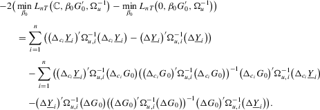
Proof of Theorem 2.3.Here,  . Let Assumption 2.1 hold and
  . By definition, we have

 (A.6)
(A.6) such that
  for some constant M. The proof of (A.6) is available in the following subsection.
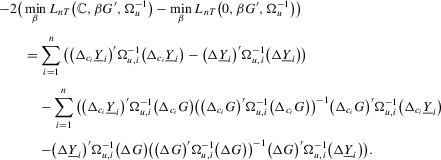
Proof of Theorem 2.5.Here,  . Let Assumption 2.1 hold and
  . By definition, we have

 (A.7)
(A.7) such that
  for some constant M. Then, we have
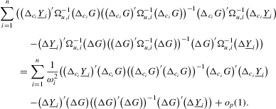

A.1 Supplementary results
A.1.1. A useful lemma
 (where
  denotes the maximum eigenvalue),
  and
and  (where
  is the
  th element of A). It is well known that

 is
is  . Let
. Let  be the
  matrix whose
  element
  is
is  if
if  and zero, if
  . Let
. Let
 (A.8)
(A.8)Lemma A.1.Let Assumption 2.1 hold. Then,  for some constant M.
Proof.For the desired result, we show


 under Assumption 2.1 and by the triangle inequality.
First, we show that  . Define
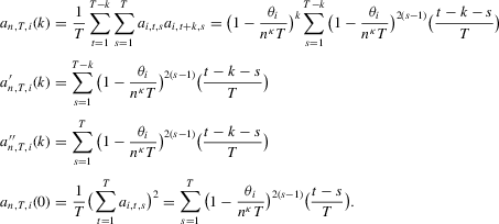

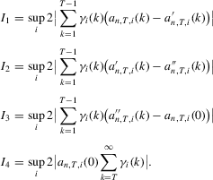

 , we have
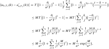
 , the last inequality uses
  and
and  and the equality uses the Taylor representation of the exponential function. Then,

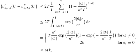
 and
and  and the last inequality holds by the mean-value theorem and
  . Then,


 . Finally, we have
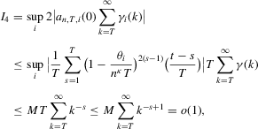

 , we have the required result

 follows in a similar fashion and is omitted.
Proof of (A.5).We prove the required result when  and
and  . Because

 (A.9)
(A.9) (A.10)
For A.9, we follow similar arguments used in proving  on p. 831 (in the proof of Lemma A2) of Elliott et al. (1996), and have for some constant M

 and by Lemma A.1, and the last inequality holds because
For A.10, we also follow similar arguments to those used in proving  on p. 831 (in the proof of Lemma A2) of Elliott et al. (1996), and have for some constant M

Proof of (A.4).We prove the required result when  and
and  . By replacing
  in
in  with
with  , we can decompose
  as
as


 , we can show that

 , we show
 (A.11)
 , the desired result follows. Because
  , we have

 , we have
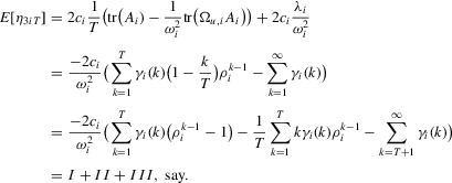
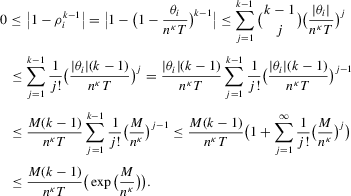
 , we can bound


 , as required.
A.1.2. More preliminary results
In this section,  and let Assumption 2.1 hold. Define
  to be the
  matrix whose
  th element is
  , where
  is defined in Assumption 2.1.
 . Direct calculations show that
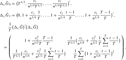
 (A.12)
 is the tth element of the vector x and
Lemma A.2.(a)  for all k; (b)
  for some finite constant M.
Proof.Part (a). By definition, for 

 , we have

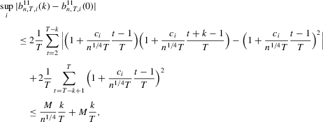
Part (b). By definition,

Lemma A.3.Suppose that  and
and  are
are  vectors such that
  is bounded, where
  is the (t)th element of
  . Then, (a)
  ; (b)
; (b)  , where
  is defined in A.8.
Proof.Part (a). The proof is similar to that of Lemma A1 of Elliott et al. (1996) and is omitted.
Part (b). We replace  in the proof of Lemma A.1 with
  . Then, the required result follows if we show

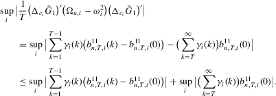
For Part (b1), by definition, we have


For Part (b2), we have


 , we define

 to be the
  th element of
  and
and  to be the kth element of
  , where
  . Similarly, we define
  and
and  .
.
Lemma A.4.Under Assumptions 2.1, the following hold: (a) 
 ; (b)
; (b)  ,
,  ; (c)
; (c)  ,
,  ; (d)
; (d)  ,
,  ; (e)
; (e)  ; (f)
; (f)  ; (g)
; (g)  .
.
Proof.Part (a). A direct calculation shows that  . We bound
  by
by
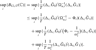


Part (b) is an immediate corollary of Part (a).
Part (c). First, note that under Assumption 2.1 we have

 . It follows immediately that

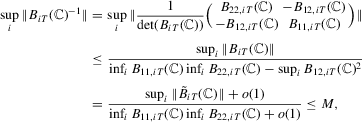
Part (d). The desired result  follows from (A.12) and by direct calculation. For the second desired result, note that
  . First,
  since
since  by
by  and by Part (g), which we prove later. Next, by definition,

 , where
  is defined above Lemma A.1, we have


Part (e). Note that


Part (f) follows by Lemma A.3(b2).
Part (g). By definition, we have

 where
where  is defined above Lemma A.1, and
  is defined in A.8 :


 and
and  we have the desired result for Part (g).
Proof of (A.6).The required result follows if we show

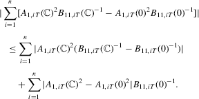

 . The second term is bounded by

 , and the last equality holds because
  . Combining these two, we have the required result


Proof of (A.7).The required result follows, if we show
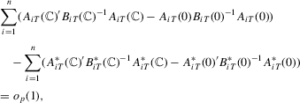
- Step 1. We show
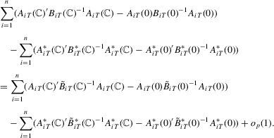
- Step 2. By (A.6), we have
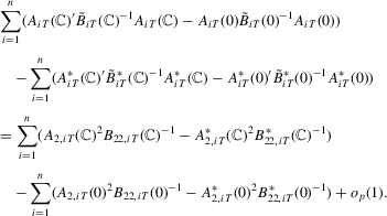
- Step 3. We show

Proof of Step 1.Note that because  is a diagonal matrix,


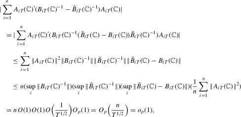


Proof of Step 3.We show

 follows in similar fashion and we omit the derivation. Note that
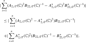

 . For the second term, note that
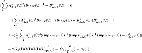
 . Then, we have all of the desired results for Part (c).
APPENDIX B:: PROOFS OF THE LIMIT DISTRIBUTION RESULTS, THEOREMS 2.2, 2.4 AND 2.6
In this section, we provide proofs of Theorems 2.2, 2.4 and 2.6. These proofs are very similar to the proofs of the corresponding results in MPP and therefore we provide just an outline of the proofs here.
Proof of Theorem 2.2.Because  , we can write
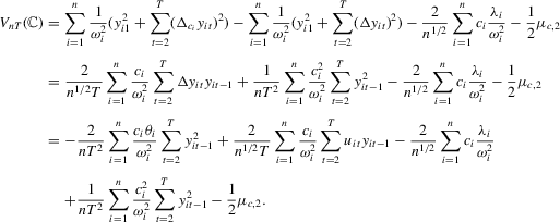


Proof of Theorem 2.4.For the required result of the theorem, it is enough to show that

 . Then,
  , and we can rewrite
  as
as


 with
with  , which proves the desired result.
Proof of Theorem 2.6.The required result is a consequence of Lemmata A.5 and A.6. 
Lemma A.5.Let Assumption 2.1 hold. Then, as  with
with  , we have
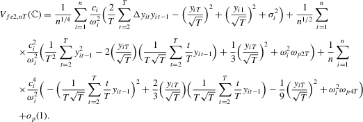
Proof.The proof is similar to the proof of Lemma 11 of MPP and is omitted. 
Proof.The proofs of Parts (b) and (c) are similar to those of Lemma 12(b) and (c) of MPP, and are omitted.
Part (a). First, note from


 we have


APPENDIX C:: PROOF OF THEOREM 2.7
Proof of Theorem 2.7.We provide a sketch of the proof. Note that under Assumption 2.2, the following hold:

 and
and  Then,
Then,


 under Assumption 2.1, we have

 satisfies the properties in Lemmata 8, 10 and 14 of MPP, while
  and
and  satisfy the properties in Lemmata 8(a), 8(b), 10(a) and 14(a)–(d) of MPP. The desired results follow by similar arguments to those used in Theorems 8, 10 and 15 of MPP.


 as
as  . Then, under the local alternative
  , we have


 with
with  we have
  ,
,  and
and  under the local alternative.
 with
with  the following hold:


