Evaluation of single and dual crop coefficients over a drip-irrigated Merlot vineyard (Vitis vinifera L.) using combined measurements of sap flow sensors and an eddy covariance system

Study site

The study site was a drip-irrigated Merlot (Vitis vinifera L.) vineyard located in the Talca Valley, Maule Region, Chile (35°25′ LS; 71°32′ LW; 125 m.a.s.l.) during the 2007/08 and 2008/09 vine growing seasons. The Merlot grapevines (grafted on 101-14 Mgt) were planted (1999) in north-south rows with a distance between and within rows equal to 2.5 m and 1.5 m, respectively. The vines were trained on VSP with the main wire 1 m above the soil surface. Grapevines were irrigated daily using drippers of 4 L/h. Also, shoots of the grapevines were maintained in a vertical plain by three wires, with the highest one located 2 m above the soil surface.

The climate is Mediterranean semi-arid with an average daily temperature of 17.1°C and a mean annual rainfall of 679 mm. The summer period is usually dry and hot (2.2% of annual rainfall) while the spring is wet (16% of annual rainfall). The soil at the vineyard is classified as Talca series (fine, mixed, thermic Ultic Haploxeralfs) with a clay loam texture and an average bulk density of 1.5 g/cm³. At effective root-zone depth (0.6 m), the volumetric soil water content at field capacity (θ_fc) and wilting point (θ_wp) were 0.36 m³/m³ and 0.22 m³/m³, respectively (Table 1).

Complementary field measurements

Irrigation was scheduled considering a maximum allowed depletion (MAD) of 0.29 m³/m³ at the effective root-zone depth. The volumetric soil water content at the root-zone depth (θ_rd) was monitored weekly at 12 sampling points distributed inside the vineyard using a portable time domain reflectometry (TDR) unit (TRASE, Soil Moisture Corp., Santa Barbara, CA, USA). Furthermore, volumetric soil water content of the upper soil layer (0.1 m) was continuously monitored using a soil water content reflectometer (CS615, Campbell Scientific Inc., Logan, UT, USA).

Vine water status was evaluated weekly using the midday stem water potential (ψ_x) measured by a pressure chamber (PMS600, PMS Instruments Company, Corvallis, OR, USA). The ψ_x was measured on 12 young, fully expanded leaves (two leaves per vine), wrapped in aluminium foil and encased in plastic bags at least 2 h before measurement (Choné et al. 2001). This parameter was used to evaluate the level of water stress in the vineyard (Williams and Trout 2005, Sibille et al. 2007).

The average fractional cover (f_c) of the vineyard was estimated ten times during each season by measuring the projected area occupied by the vine (fraction of ground shaded by the vertical projection of the canopy at midday), using digital images. The analysis of the digital images (white and black pixel count) was made using a script written in MATLAB® 2009a (The Mathworks Inc., Natick, MA, USA).

Sap flow measurements

Vine transpiration (T_sap) was determined using sap flow sensors (700 SF-100, Tranzflo, Palmerston North, New Zealand) inserted in the trunk of eight vines (one sap flow sensor per vine), with a similar trunk diameter near to the EC system. Vine canopy transpiration was determined by the compensated heat-pulse velocity method (Green et al. 2003, Alarcon et al. 2005, Poblete-Echeverría et al. 2012). The upstream sensor probe (x_u) was located 5 mm below the heater probe, and the downstream sensor (x_d) was located 10 mm above the heater probe. On each sensor, there are three thermistors, positioned at 5 mm, 10 mm and 15 mm. A data logger (CR23X, Campbell Scientific Inc., Logan, UT, USA) was used to trigger heat pulses and record the time interval between the initiation of a heat pulse and equilibration between upstream and downstream temperature (t_z). Heat pulses of 0.75 s were automatically triggered every hour throughout the day. For this experiment, the sap flow measurements were evaluated by Poblete-Echeverría et al. (2012) using residual transpiration (T_r) obtained by combined measurements of the EC system and microlysimeters. This study showed a good agreement between T_sap and T_r with a root mean square error (RMSE) equal to 0.22 mm/day when a correction coefficient for a wound size of 2.4 mm was applied.

Meteorological measurements

ET_o (mm/day) was calculated by the FAO-56 Penman–Monteith equation (Allen et al. 1998):

(1)

where Rn_grass is the net radiation above a grass surface (MJ/m²day), G_grass is the soil heat flux (MJ/m²day), T_a is the air temperature at 2 m height (°C), u₂ is the wind speed at 2 m height (m/s), e_s is the saturation vapour pressure (kPa), e_a is the actual vapour pressure (kPa), Δ is the slope of the vapour pressure curve (kPa/°C) and γ is the psychrometric constant (kPa/°C). To calculate the ET_o, daily values of T_a, Rn_grass, u₂ and relative humidity (RH) were collected from a nearby automatic weather station (35°37′ LS; 71°59′ LW; 118 m.a.s.l.). A second automatic weather station was installed within the vineyard for measuring conventional meteorological variables. Also, precipitation (PP) was measured at both stations. The value of mean daily air temperature measured in the vineyard (T_av) was used to calculate cumulative growing degree days (GDD) using a 10°C base.

Micrometeorological measurements

ET_a was obtained using an EC system (ET_{a_ec}) installed 4.7 m above the soil surface. Fluxes of latent (LE) and sensible (H) heat were registered with an infrared gas analyser (LI-7500, Li-Cor Biosciences, Lincoln, NB, USA) and a sonic anemometer (CSAT3, Campbell Scientific Inc., Logan, UT, USA). Vineyard soil heat flux (G) was measured by eight soil heat flux plates of constant thermal conductivity (HFT3, Campbell Scientific Inc., Logan, UT, USA) and four pairs of thermocouples. The heat stored above the plates was added algebraically to the fluxes measured by the flux plates (Ortega-Farias et al. 2010). Net radiation over the vineyard (Rn) was measured at 4.7 m by a four-way net radiometer (CNR1, Kipp & Zonen Inc., Delft, The Netherlands). The accuracy of the EC system measurements was evaluated using the energy balance ratio calculated on a daily basis. More details about the distribution and configuration of the sensors are described by Poblete-Echeverría and Ortega-Farias (2009).

Single and dual crop coefficient using the FAO-56 approach

In the single crop coefficient approach, the effects of crop transpiration and soil evaporation are combined into a single coefficient (K_c). Thereby, ET_a estimated by the single crop coefficient approach (ET_{a_sc}) expressed in mm/day is calculated by the following equation:

(2)

On the other hand, in the dual crop coefficient approach, the effects of crop transpiration and soil evaporation are determined separately. K_c is split into two separate coefficients K_cb and K_e. In this case, ET_a estimated by the dual crop coefficient approach (ET_{a_dc}) expressed in mm/day is estimated using the following equation:

(3)

where K_cb and K_e are the basal and soil evaporation coefficients, respectively.

Following the segment approach proposed by the FAO-56, the vine growing seasons were divided into four growth stages: (i) the initial stage (L_ini); (ii) crop development stage (L_dev); (iii) midseason stage (L_mid); and (iv) late season stage (L_late). L_ini and L_mid are characterised by horizontal line segment while L_dev and L_late are characterised by rising and falling line segments, respectively (Figure 5). A piecewise line function (SigmaPlot v12.0; Systat Software GmbH, Erkrath, Germany) was used to obtain the average value of K_c and K_cb at the initial, midseason and late growing stage. The FAO-56 and observed length of growth stages for the vineyard are given in Table 2. In the segment approach, three critical K_c and K_cb values are required to generate the entire K_c and K_cb curves during the vine growing season. The recommended values of K_c and K_cb presented by Allen et al. (1998) for the different vine development stages are given in Table 3.

For the dual crop coefficient approach, K_e based on the daily water balance for the surface soil evaporation layer is calculated by the following equation:

(4)

where K_r is the evaporation reduction coefficient (dimensionless), f_ew is the fraction of the soil wetted and exposed (dimensionless), and K_cmax is the maximum value of K_c. K_{c max} is calculated by the following equation:

(5)

where RH_min is the minimum RH (%) measured over a grass surface, u₂ is the average wind speed measured at 2 m (m/s), and h is the average vine height (m). K_r is calculated by the following equation:

(6)

(7)

where TEW is the total evaporable water (mm), Z_e is the depth of soil surface layer (m), REW is the readily evaporable water (mm), and D_e is the evaporation depletion (mm). Table 1 shows the input soil parameters used in the calculation of K_r.

On the other hand, the single and dual crop coefficients calculated using measurements from the EC system and sap flow sensors were obtained by the following equations:

(8)

(9)

(10)

where K_{c_ec} is the single crop coefficient calculated using ET_a obtained from the EC system; K_{cb_sap} is the basal crop coefficient calculated using sap flow measurements; and K_{e_sap} is the soil evaporation coefficient calculated as the difference between ET_{a_ec} and T_sap (residual soil evaporation (Eec_sap)) divided by ET_o. Values of ET_{a_ec}, T_sap and ET_o are expressed in mm/day.

Statistical analysis

In this study, ET_a was computed by three approaches: (i) using K_c values and length of growth stages (L) values recommended by the FAO-56 (ET_{a_sc} FAO-56 = K_c ET_o); (ii) using dual crop coefficients and L-values recommended by the FAO-56 (ET_{a_dc} FAO-56 = (K_cb + K_e) ET_o); and (iii) using K_{cb_sap} and observed values of L (ET_{a_dc} SAP = (K_{cb_sap} + K_{e_sap}) ET_o). Recommended and observed values of L, single and dual coefficients are indicated in Tables 2 and 3. Computed ET_a values were compared with those obtained by the EC system (ET_{a_ec}). The statistical comparison included a linear regression analysis, the RMSE, mean absolute error (MAE), model efficiency (EF) and index of agreement (d) (Table 4) (Willmott 1982, Mayer and Butler 1993, Legates and McCabe 1999).

Table 4. Statistical parameters and criteria for evaluating the performance of three approaches used to compute actual evapotranspiration of the Merlot vineyard

Statistical parameters	Symbol	Equation	Optimum
Root mean square error	RMSE		0
Mean absolute error	MAE		0
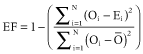
Model efficiency	EF		1
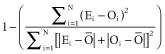
Index of agreement	d		1

• where N is the total number of observations, E_i and O_i are the estimated and observed values, respectively, and is the mean of the observed values.

Weather conditions

Growing seasons experienced in this study were dry and hot with average air temperature (Ta) equal to 18.5°C during the 2007/08 season and 19.6°C during the 2008/09 season. The average daily value of the vapour pressure deficit (VPD) was similar during both seasons at around 1.0 kPa. Maximum values of VPD were around 1.6 kPa during the first season and 1.8 kPa during the second season (Figure 1). The average value of wind speed (u) was 0.9 m/s and 1.36 m/s for the first and second seasons, respectively. Temporal patterns of rainfall over both vine growing seasons were characterised by low and irregular rain events, with a total PP amount (from DOY274 to DOY100) of 11.6 mm during the 2007/08 season and only 3.2 mm (from DOY271 to DOY89) during the 2008/09 season.

Soil and plant water status

The average value of θ_rd measured by TDR was similar during both seasons, with an average around 0.31 m³/m³ (Figure 2). This soil moisture value is an indication that the Merlot vineyard was well irrigated, with θ_rd maintained between θ_fc and MAD levels. The average value of ψ_x ranged between −0.42 and −1.0 MPa and −0.66 and −1.1 MPa during the first and second season, respectively (Figure 2). These values showed that the Merlot vineyard was not under water stress during the study period (Williams and Trout 2005, Sibille et al. 2007).

Surface energy balance closure

Based on the first law of thermodynamics (conservation of energy), the accuracy of the EC system to measure turbulent fluxes was evaluated using the energy balance closure, which is a linear regression between turbulent energy fluxes (H + LE) and available energy (Rn−G) (Baldocchi et al. 2000, Twine et al. 2000, Wilson et al. 2002). Figure 3 shows the energy balance closure over a drip-irrigated Merlot vineyard for the 2007/08 and 2008/09 seasons. This figure indicates that the comparison points were close to line 1:1, presenting an acceptable energy balance closure with a slope passing through the origin (b) equal to 0.88 for both seasons. Also, the value of the determination coefficient (r²) was 0.95 and 0.88 for the first and second seasons, respectively. The analysis of surface energy balance closure indicates that the turbulent fluxes were about 12% less than the available energy for the two seasons. This value represents a good energy balance closure, which is in agreement with other studies that present a lack of energy balance closure between 10 and 30% (Baldocchi et al. 2000, Twine et al. 2000, Testi et al. 2004). Similar results were found by Spano et al. (2004) and Poblete-Echeverría and Ortega-Farias (2012) who indicated an imbalance of 16% and 11% for drip-irrigated Sangiovese and Merlot vineyards, respectively.

Reference and ET_a

Seasonal variations of ET_o and ET_{a_ec} are shown in Figure 4 for the 2007/08 and 2008/09 seasons, respectively. These figures shows that the ET_o temporal pattern is typically associated with a semi-arid climate belonging to the southern hemisphere, which is characterised by a high ET_o value in December with a maximum value of 7.3 mm/day during the first season and 6.9 mm/day during the second season (Table 5). Accumulated ET_o for the first (between DOY274 and DOY100) and second (DOY271 and DOY89) seasons were 839.1 and 872.3 mm, respectively. Furthermore, the ET_{a_ec} value measured by the EC system ranged from 2.0 mm/day, early in the season, when the shoots were growing, to a value of around 5 mm/day when vines reached full cover (f_c ≈ 30%). The mean ET_{a_ec} value obtained in this study was 2.6 mm/day during the first season and 2.9 mm/day during the second season (Table 5). These values are in agreement with those reported in literature for grapevines (Oliver and Sene 1992, Evans et al. 1993, Trambouze et al. 1998, Yunusa et al. 2004, Williams and Ayars 2005, Ortega-Farias et al. 2010).

Single crop coefficient

Observed K_c values (K_{c_ec}) for the vineyard were obtained using Equation 8. At the initial stage of crop growth (K_{c_ec_ini}), the value was low, but increased with crop development and remained almost constant at full canopy cover (Table 3). Recommended (K_{c_ini}, K_{c_mid} and K_{c_late}) and observed values (K_{c_ec_ini}, K_{c_ec_mid} and K_{c_ec_late}) are presented in Table 3. The mean value of observed K_{c_ec} at the initial stage for the 2007/08 and 2008/09 seasons was higher than that recommended by the FAO-56 (K_{c_ini} = 0.30). On the contrary, K_{c_ec_mid} for the 2007/08 and 2008/09 seasons (0.60 and 0.64) were lower than those recommended by FAO-56 (K_{c_mid} = 0.70) (Table 3). This lower K_{c_ec} value at the mid-growth stage is attributed to low fractional cover (f_c ≈ 30%) observed in this study. In this regard, Allen and Pereira (2009) proposed new values of K_{c_mid} for grapevines depending on fractional cover and height, corresponding to a K_{c_mid} of 0.64 (no stress conditions) and a K_{c_mid} of 0.45 (for stressed vines with a stress coefficient of 0.7) for low density grapevines (f_c = 25%). Similar results were observed by Montoro et al. (2008), who reported a monthly mean K_c around 0.65 at peak vegetation cover for daily drip-irrigated grapevines cv. Cencibel using a weighing lysimeter. In addition, Williams and Ayars (2005) developed a linear relation for Thompson Seedless to obtain a single crop coefficient as a function of f_c (K_c = −0.008 + 0.017f_c). This approach has a strong practical implication because techniques for the measurement of f_c and leaf area index (LAI) have been advanced lately using digital imaging analysis (e.g. Fuentes et al. 2008). Finally, the values of K_{c_ec_late} obtained in this study were 0.58 and 0.53 for first and second seasons, respectively. These values were higher than those recommended by the FAO-56 (K_{c_late} = 0.45).

Also, in seasonal terms, ET_{a_ec} presented a significant linear relationship with ET_o (Figure 4). The linear regression obtained (forced to pass through the origin) between ET_{a_ec} and ET_o presented a determination coefficient (r²) of 0.76 and a slope (b) of 0.58 for the first season and r² equal to 0.69 and b equal to 0.61 for the second season. In this case, b-values represent a whole value of K_{c_ec} which are similar to average values at the midgrowth stage (Table 3).

Dual crop coefficient

Vine transpiration measured by sap flow sensors (T_sap) ranged between 1.2 and 3.4 mm/day for the first growing season with a mean value of 2.2 mm/day. In the second season, the T_sap value ranged between 0.3 and 4.3 mm/day with a mean value of 2.4 mm/day (Table 5). These results are similar to those registered by other studies (Eastham and Gray 1998, Yunusa et al. 2004). Also, T_sap values presented a significant linear relationship when compared with ET_o values (Figure 6). The linear regression obtained (forced to pass through the origin) between T_sap and ET_o presented a determination coefficient (r²) of 0.75 and a slope (b) of 0.47 for the first season and r² equal to 0.64 and b equal to 0.50 for the second season. These results are in accordance with other studies, which found a linear relationship between T_sap and ET_o for well-irrigated olive trees (Fernández et al. 2001, Rousseaux et al. 2009), apricot trees (Nicolas et al. 2005) and lemon trees (Ortuño et al. 2006).

In this study, T_sap values were used to calculate new critical values to generate the entire K_cb curve during the whole vine growing season. Figure 5 shows a comparison between recommended and observed K_cb curves for the different growth stages: initial (K_{cb_ini}, budburst to 10% of full effective cover), development (K_{cb_dev}, 10% of full effective cover), midseason (K_{cb_mid}, from full effective cover to full maturity) and late season (K_{cb_late}, from full maturity to harvest of grapes). From Figure 5a, it can be seen that the observed K_cb at the initial growth stage (K_{cb_ini} = 0.27) is higher than that recommended by the FAO-56 (0.15). Also, the value of K_{cb_mid} (0.55) is lower than that recommended by the FAO-56 (0.65). Finally, the value of K_{cb_late} (0.43) is slightly higher than that recommended by the FAO-56 (0.40). Similar differences were found in the second season (Figure 5b) where the observed values of K_{cb_ini}, K_{cb_mid} and K_{cb_late} were equal to 0.20, 0.55 and 0.43, respectively. Following, the approach proposed by Williams and Ayars (2005) for obtaining a single crop coefficient, sap flow sensors could be used to characterise K_cb and relate them to f_c or LAI for obtaining site-specific relation between these variables.

The length of the Merlot vineyard growth stages during the 2007/08 and 2008/09 seasons is shown in Table 2. The length of the initial growth stage (L_ini) was between 31 and 38 days, which differed by 1 and 8 days more than the length considered by the FAO-56. The developing growth stage, however, was shorter than that considered by the FAO-56 for both study seasons with a difference of 13 and 19 days for the 2007/08 and 2008/09 seasons, respectively. The midseason growth stage observed in this study was significantly longer than the length considered by the FAO-56 with a difference of 23 and 22 days for the first and second seasons, respectively. The length of the late growth stage (L_late) was 30 and 38 days shorter than values considered by the FAO-56. Finally, the total length of the vine growing season observed in this study was 192 and 184 days for the 2007/08 and 2008/09 seasons, respectively. These values were shorter than those suggested by the FAO-56 (210 days) with a difference of 18 for the 2007/08 season and 26 days for the 2008/09 season. The differences in the length of growing stages between the experimental seasons compared with those considered in the FAO-56 may be attributed to climatic conditions at the study site. In this regard, several recent studies have reported that climate change is expected to have a significant impact on the length of the growing season because of an increased temperature (Jones et al. 2005, Webb et al. 2007, Caffarra and Eccel 2011, Tomasi et al. 2011). Webb et al. (2007), using warming projections based on future greenhouse gas emission scenarios and patterns of climate change, reported that season duration (from budburst to harvest) will be compressed in all Australian vineyard regions resulting in early harvests. In Chile, this effect is not clear because of the influence of the ‘El Niño-Southern Oscillation’ (ENSO). ENSO events include Niño events, which are characterised by high rainfall and moderate temperatures, and Niña events that produce the opposite effects, droughts and high temperatures.

One problem in determining the length of growth stages in chronological time is that data are not transferable to other agro-climatic locations. One solution is to express K_cb curves in terms of GDD (de Medeiros et al. 2001). GDD values for the two study seasons are presented in Table 2. The second season shows slightly more cumulative GDD than the first season, completing the vine growth in less time. The cumulative GDD in the total vine growth periods, however, was similar for both seasons (Table 2). The differences between seasons with respect to the length of growth stages can be explained by the changes in climatic conditions during specific periods. In the season 2007/08 (Niña), the bud-break was 6 days after that of the 2008/09 season (normal).

The average value of E_{ec_sap} found in this study was similar during both seasons. In the first season, the E_{ec_sap} value ranged from 0.1 to 1.3 mm/day with an average value of 0.6 mm/day. In the second season, the E_{ec_sap} value ranged from 0.1 to 1.3 mm/day with an average value of 0.5 mm/day (Table 5). The ratio of E_{ec_sap} to ET_a found in this study was 0.23 during the first season and 0.17 during the second season. Also, the whole evaporation coefficient calculated by a lineal regression analysis was 0.12 and 0.11 for first and second season, respectively. Unlike what happened with the relation between ET_o and ET_{a_ec}, the r² value in the relation between ET_o and E_{ec_sap} was low with values of 0.38 and 0.26 for the first and second season, respectively (Figure 6). A low r² value can be related to a low (mean value less than 0.6 mm/day), and relatively constant (standard deviation less than 0.31 mm/day) value of soil evaporation. In the same experimental plot, values of E_s measured by microlysimeters were reported by Poblete-Echeverría et al. (2012) who indicated that the E_s value ranged from 0.28 to 1.14 mm/day during the season 2007/08 and from 0.37 to 1.04 mm/day during the 2008/09 season.

E_{ec_sap} values calculated in this study are similar to those found by Yunusa et al. (2004) in Australia, who presented an average value of 0.4 mm/day in a drip-irrigated Sultana vineyard in a dry period (no rainfall or irrigation events), which corresponds to 21% of ET_a and only 3% of ET_o. For the irrigated period, Yunusa et al. (2004) found an average value of E_s of 1.6 mm/day which represents 26 and 64% of ET_o and ET_a, respectively. For a partial root-zone, furrow-irrigated Merlot vineyard in China, Zhang et al. (2009) indicated that the value of E_s measured by microlysimeters was around 2.2 mm/day for the 6 consecutively days after irrigation. In Brazil, Teixeira et al. (2007) found that for drip-irrigated grapevines cv. Petite Syrah, E_s was from 8 to 9% of ET_o and from 11 to 12% of ET_a. In the same study, for the table grape cv. Superior Seedless with microsprinkler irrigation E_s was from 15 to 19% of ET_o and from 17 to 21% of ET_a.

Estimation of ET_a

Figure 7 shows the comparison between ET_{a_ec} and ET_a simulated by the three approaches studied (ET_{a_sc} FAO-56, ET_{a_dc} FAO-56 and ET_{a_dc} SAP). In the first season when recommended values of K_c are used, the single crop coefficient approach (ET_{a_sc} FAO-56) tended to overestimate ET_{a_ec} (Figure 7a). In the second season, however, the comparison between ET_{a_sc} FAO-56 versus ET_{a_ec} (measured value) was improved, with points close to 1:1 line (Figure 7b). Likewise, when recommended values of K_cb and L are used, the dual crop coefficient approach tended to overestimate ET_a especially for high values (over 3 mm/day) (Figure 7). When the observed values of K_cb and L are used (ET_{a_dc} SAP), however, the dual crop coefficient approach shows that points were uniformly distributed around the 1:1 line (Figure 7).

Figure 8 shows a seasonal daily comparison between ET_a observed and calculated by the three approaches studied from DOY326 to DOY99 for the first season and from DOY296 to DOY89 for the second season. There is good agreement between observed and estimated ET_a values during both vine growing seasons. Some discrepancies between observed and simulated ET_a values can be seen after rainfall events and stress periods in the first season (Figure 8a).

For rainfall events, the difference between measured and simulated ET_a values may be explained by uncertainties in the measurements of the EC system (Er-Raki et al. 2010) and by problems associated with the estimation of soil evaporation, when the soil surface reaches water saturation after the rainfall event. This effect is corroborated by Liu and Luo (2010) who found that the dual approach of the FAO-56 is appropriate for estimating the total quantity of evapotranspiration, but inaccurate when simulating the peak value after PP or irrigation.

The summer period in Chile is characteristically dry. So, in this study, only one rainfall event of 7.6 mm (season 2007/08) produced an underestimation of ET_{a_ec} of about 23% in the case of the ET_{a_dc} SAP approach; 19% in the case of the ET_{a_sc} FAO-56 approach; and 15% in the case of ET_{a_dc} FAO-56. In general, the experimental plots were well irrigated, however, near veraison, the ψ_x reached values lower than −1.0 MPa (Figure 2), which indicated a mild stress for this period. This stress level could lead to the dual crop coefficient approach overestimating ET_a compared with the EC system because of an overestimation of the soil water stress coefficient (Er-Raki et al. 2010). For example, for the stress period of the first season (DOY17 to DOY26), the single crop coefficient approach using recommended values of K_c and L tended to overestimate ET_{a_ec} by about 22%; the dual crop coefficient approach using recommended values of K_cb and L tended to overestimate ET_{a_ec} by about 26% and the dual crop coefficient approach using observed values of K_cb and L tended to overestimate ET_a by only 3%.

The performance of single and dual crop coefficient approaches to estimate ET_a over daily periods is shown in Table 6. The statistical analysis indicates that the single crop coefficient approach using recommended values of K_c and L was able to predict ET_{a_ec} with overall values of r², EF and d equal to 0.83, 0.78 and 0.95, respectively. So, the single crop coefficient approach using recommended values of K_c and L produces a good estimation of ET_{a_ec} with a low absolute error 0.35 mm/day (12.8% error). In the case of dual crop coefficient approach using recommended values of K_cb and L, the statistical analysis presented in Table 6 shows that this approach had a lower agreement with values of ET_{a_ec} showing overall values of r², EF and d equal to 0.86, 0.52 and 0.91, respectively. Also, the overall values of RMSE and MAE were 0.69 mm/day (24.8% error) and 0.54 mm/day (19.6% error), respectively (Table 6). However, the dual crop coefficient approach using observed values of K_cb and L showed the best estimation of ET_{a_ec} with overall values of r², EF and d equal to 0.87, 0.86 and 0.96, respectively. Also, overall values of RMSE and MAE were, respectively, 0.37 (13.2% error) and 0.28 mm/day (10.3% error) (Table 6). This analysis indicated that the use of sap flow sensors for obtaining site-specific K_cb values in the dual crop coefficient approach reduces the RMSE values from 0.69 to 0.37 mm/day (46% of error reduction) and MAE values from 0.54 to 0.28 mm/day (48% of error reduction).

Recent studies in orchards have shown a good correlation between ET_a estimated by the dual crop coefficient approach and ET_a measured by the EC system. For example, Paco et al. (2006), using an EC system in a peach orchard, found a good correlation with a slope of 0.77 and r² equal to 0.73. Using the same comparison method in an olive orchard, Er-Raki et al. (2010) found that the dual crop coefficient approach estimated ET_a with an RMSE of 0.54 and 0.71 mm/day for the 2003 and 2004 seasons, respectively. Several studies, however, have emphasised the need to calibrate the K_cb values by comparing them with measurements obtained locally (Carr 2001, Flumignan et al. 2011). Dragoni et al. (2004), in an apple orchard, showed a significant overestimation (over 15%) of K_cb by the FAO-56 method compared with sap flow measurements. Paco et al. (2006) calculated a mean K_cb of 0.5 which is less than that suggested by the FAO-56 for peach orchards (K_cb = 0.7).