Fund Volatility Index using equity market state prices
Abstract
The Fund Volatility Index (FVX) is proposed as a forward measure of volatility with applications in fund hedging and risk management. The method applies equity market state prices to individual fund pay-offs. FVX is validated as a predictor of short-term realised volatility for 30 exchange traded funds. Performance of the method is compared with existing methods using a data set of 14 925 non-traded funds. FVX has lower bias and higher forecast accuracy than existing methods. As a more general measure, it allows for incorporation of terms to capture individual fund skewness and projection of higher moments of returns.
1 Introduction
The Chicago Board Options Exchange (CBOE) VIX is the most prevalent forward-looking measure for volatility and is available in real time (Whaley, 2009). Mutual funds would benefit from a fund-specific forward volatility index, available intraday like the VIX. Such forecasts are relevant to short-term investment, hedging and risk management decisions, including the pricing of portfolio insurance for individual funds.1 Moreover, forecasts are also important for market timing decisions made by both mutual funds and the individuals who invest in them.2
Available fund volatility measures include the historic average, autoregressive conditional heteroskedasticity or ‘ARCH’ (Engle, 1982), generalised autoregressive conditional heteroskedasticity or ‘GARCH’ (Bollerslev, 1986; Engle and Kroner, 1995), and exponentially weighted moving average or ‘EWMA’ volatility (Holt, 1957; Winters, 1960). Engle (2001) has applied these methods in assessing portfolio value at risk, portfolio selection and derivative pricing. However, the existing methods prove to be unreliable predictors of future volatility (Cumby et al., 1993; Jorion, 1995, 1996; Figlewski, 1997).3
This study proposes a Fund Volatility Index (FVX) tailored for individual funds from theoretical equity market state prices to meet this need.
Existing empirical models of volatility are deficient in that they are not supported by theory. Poon and Granger (2003) review the prevailing time series models for volatility, observing that models developed to capture persistence, clustering and asymmetry of volatility do not have a theoretical basis. Unlike existing models, the FVX is based on the most celebrated theoretical foundations in all of financial economics, the state pricing theory of Debreu (1959) and Arrow (1964).4 The development of the FVX is proposed using state prices derived from the S&P 500 options market to value contingent claims by mutual funds on the market. State prices are derived using similar methodology to that applied by Barraclough (2007). The novelty lies in application of market state prices to price the volatility of individual funds and to develop the FVX. The formulation is available in real time and does not rely on up-to-date valuations of fund assets.
The FVX is applied to generate forecasts of 22-day forward volatility at the individual fund level, similar to the VIX. Performance is assessed using a regression of short-term realised volatility on forecast volatility. Overall, the results suggest that the FVX is efficient and unbiased as a projector of realised fund volatility. The generality of the method allows the incorporation of additional terms, such as the upper versus lower partial moment, which may be useful in capturing the asymmetric return distributions of some funds. There is also the potential to extend the method in order to project higher moments of the fund return distribution or project tail risk using a contingent pay-off that is out of the money.
The study is organised as follows. Section 2 summarises the empirical methodology used to generate the FVX. Section 3 demonstrates the application to 30 exchange traded funds (ETFs). Section 4 assesses the performance of the FVX across a large sample of non-traded funds, and the last section summarises the results of the study.
2 Calculation of the Fund Volatility Index
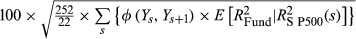
 (1)
(1)In the application of these methods to equity markets, each market state price  is defined as the price of a security that pays off 1 when the market is up by
  and 0 elsewhere in increments Ys, Ys + 1, with Ys + 1 > Ys.
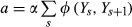
 (2)
(2) is the expected pay-off for the fund conditional on the level of the index. The fund pay-off here is the expected squared log returns
  .
. (3)
(3) ;
;T = (22/252) with 22 trading days per month; r is the risk-free rate;
 ;
;
PVD is the present value of dividends; and
σ is the volatility input.
In the calculation of these measures, the maximum and minimum values of Y are bounded between 215 and 2348, being 50 percent below the minimum and 50 percent above the maximum, respectively, over the period 1998 to 2009. State prices are assessed in increments of 1 between Ys and Ys + 1, representing 1 index point on the S&P 500. The volatility input is based on implied volatility from the option market, rather than alternatives such as the VIX or realised volatility measures. The input is calculated by interpolating between the closest to the money put and call option strike prices straddling the spot level of the S&P 500 Index.6
Implied volatilities of individual options are calculated using the mid-point of the best closing bid and best closing offer price for the option, with data obtained from the OptionMetrics database, provided by Wharton Research Data Services (WRDS: http://whartonwrds.com/). The data are available from January 1996 forward. The CBOE Short-term Interest Rate Index (IRX) is used as a proxy for the risk-free rate, being based on the annualised discount rate of the most recently auctioned 13-week Treasury Bill (http://www.cboe.com/). The present value of dividends for the S&P 500 Index is calculated on a daily basis as the difference between daily returns, inclusive and exclusive of dividends, using the Centre for Research in Security Prices (CRSP) database from Wharton Research Data Services (http://whartonwrds.com/).7
 (4)
(4) (5)
(5) (6)
(6) (7)
(7) for state s;
 is the associated expected return for the fund;
 ;
;
 is the state price measure for the market;
 ; and
; and
 is the value of a risk-free asset with a pay-off of 1. Note that in Formulation 2, a is further adjusted by the price of a discount bond paying α.
There are many ways to determine  .8 This study determines
  based on a simple linear least squares regression of daily fund returns on S&P 500 market returns. The method captures the idiosyncratic components of fund volatility to the extent that the coefficient is allowed to vary over time.9 Note that the result should be exactly the same as a linear model β ×
  if the α term was excluded.
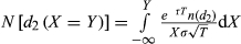
 is fitted using daily return data from the CRSP database. Fund data are available from 1 September 1998 to 31 October 2009, thus dictating the sample period. The fit is based on an expanding rather than fixed window of historic data. The results are assessed against realised volatility. In this study, realised volatility refers to close–close realised volatility in CRSP daily returns, annualised and scaled in the same way as the CBOE VIX (Whaley, 2009):
 (8)
(8)Predictive power is assessed using a linear regression of 22-day realised close–close volatility on the FVX. Statistical significance is assessed allowing for overlapping observations, using the covariance matrix of Newey and West (1987, 1994).
 (9)
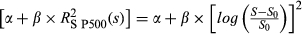
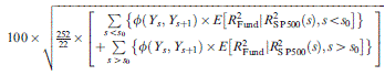
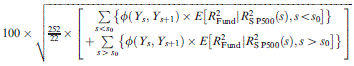
(9) In particular, individual fund returns can be skewed, while the S&P 500 Index portfolio is more diversified and likely to be less skewed.10 The generality of the FVX allows the incorporation of additional terms to capture the asymmetry of fund volatility in up- versus downmarkets, with an indicator term which represents the direction of state change. That is, FVX Formulation 1 can be augmented to incorporate the mean upper versus lower partial moment (ULPM) in the form:
 (10)
(10)An indicator term could also be included for the absolute size of a market jump, based on the distribution of intraday changes in state over a period of time. There is also potential to use the FVX to project higher moments of fund returns by applying the same market state prices to a different contingent pay-off.
3 Application to exchange traded funds
In this section, the validity of the FVX is initially demonstrated on the ETFs. For this validation, FVX Formulation 1 is used with the implied volatility input. The coefficient of  is fitted using the daily return data.
Thirty ETFs were tested, all being equity market funds with track records between 4 and 5 years. The group had an average allocation to equities of 97 percent over the period. Predictive power is assessed using a linear regression of 22-day realised close–close volatility on the FVX.
Figure 1 demonstrates the performance of the method for a selected fund, the RevenueShares Mid Cap Fund (RWK). In this case, there were 445 return data points, and the FVX was generated from 2 months after inception. In Panel A, realised volatility is calculated from daily return data and compared with forecast volatility using the FVX Formulation 1. In Panel B, the intercept and coefficient terms used to fit 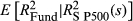 for this example are shown. Panel B also shows the upper versus lower partial moments, UPM and LPM, respectively. The intercept and coefficient terms are stable over time, demonstrating minor changes in forecast volatility at the fund level that are not related to the market. There is a significant change in coefficients on 30 September 2008, with a market correction having occurred at the beginning of that month. The difference between the upper versus lower partial moment is also stable and significant, justifying the use of the additional indicator term for this fund.

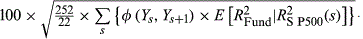
- The results of applying FVX formulation 1 from Equation 5 to RWK are shown. FVX formulation 1 is calculated as
 and fitted with an expanding window of data. The number of daily return observations available is 445. The figures exclude the first 2 months since inception. In Panel A, FVX is compared with 22-day realised fund volatility (RV), annualised and scaled in the same way as the Chicago Board Options Exchange VIX. In Panel B, the intercept and slope terms from the regression of daily fund variance on market variance are shown, excluding the first 2 months since inception. The upper versus lower partial moments (UPM, LPM) from the regression of daily fund variance on market variance are also shown, calculated as
  and
and  , respectively.
The performance of the method can be assessed using an ordinary least squares regression of realised fund volatility on the FVX. The adjusted R2 of this regression was 0.67. Statistical significance was measured using the method of Newey and West (1987, 1994), to account for overlapping observations. The intercept was not significantly different from zero, with a value of −6.20 and a t-statistic of −1.53. In this case, the estimate involved some bias relative to realised volatility. The slope had a value of 1.54 and was significantly different from 1 with a t-statistic of 3.83.
Table 1 shows the results of modelling all 30 ETFs. The average adjusted R2 of FVX Formulation 1 against close–close volatility was 0.65. The adjusted R2 of the regression exceeded 0.6 for 24 of the 30 funds. The intercept and coefficient terms used to fit  are not reported. These terms tended to be stable with very little variability over time for the vast majority of funds. That is, for most funds, idiosyncratic volatility tended to be stable.
| Fund (Ticker) | Intercept | Coefficient | Adjusted R2 | Observations |
|---|---|---|---|---|
| Grail American Beacon Large Value ETF (GVT) | 6.43 (2.91)*** | 0.5 (−7.49)*** | 0.62 | 143 |
| Guggenheim Insider Sentiment (NFO) | −5.83 (−2.91)*** | 1.41 (4.35)*** | 0.75 | 799 |
| Guggenheim Mid-Cap Core (CZA) | 0.69 (0.22) | 1.02 (0.18) | 0.57 | 668 |
| Guggenheim Raymond James SB-1 Equity (RYJ) | −10.80 (−4.30)*** | 1.09 (1.36) | 0.91 | 183 |
| Guggenheim Sector Rotation (XRO) | 0.17 (0.05) | 0.99 (−0.06) | 0.52 | 799 |
| Guggenheim Spin-Off (CSD) | 0.61 (0.21) | 1.14 (0.94) | 0.65 | 739 |
| RevenueShares Large Cap (RWL) | −3.95 (−0.84) | 1.25 (1.86)* | 0.61 | 445 |
| RevenueShares Mid Cap (RWK) | −6.20 (−1.53) | 1.54 (3.83)*** | 0.67 | 445 |
| RevenueShares Navellier Overall A-100 (RWV) | 23.68 (2.35)** | −0.32 (−0.83) | 0.00 | 299 |
| RevenueShares Small Cap (RWJ) | −5.95 (−1.56) | 1.68 (4.63)*** | 0.68 | 445 |
| Rydex 2× S&P 500 (RSU) | −10.26 (−0.86) | 1.24 (1.14) | 0.59 | 518 |
| Rydex Russell Top 50 (XLG) | −1.49 (−0.8) | 1.12 (0.83) | 0.71 | 1144 |
| Rydex S&P 500 Pure Growth (RPG) | −2.42 (−1.17) | 1.24 (1.81)* | 0.76 | 941 |
| Rydex S&P 500 Pure Value (RPV) | −6.00 (−1.66)* | 1.61 (3.31)*** | 0.78 | 941 |
| Rydex S&P Midcap 400 Pure Growth (RFG) | −6.78 (−3.16)*** | 1.54 (4.51)*** | 0.78 | 941 |
| Rydex S&P Midcap 400 Pure Value (RFV) | −3.01 (−0.39) | 1.71 (3.40)*** | 0.60 | 941 |
| Rydex S&P SmallCap 600 Pure Growth (RZG) | −0.98 (−0.09) | 1.65 (1.96)* | 0.35 | 941 |
| Rydex S&P SmallCap 600 Pure Value (RZV) | −15.37 (−6.01)*** | 2.09 (8.38)*** | 0.79 | 941 |
| SPDR Dow Jones Large Cap (ELR) | −2.50 (−1.42) | 1.15 (1.28) | 0.72 | 1016 |
| SPDR Dow Jones Mid Cap (EMM) | −3.80 (−2.40)** | 1.36 (3.43)*** | 0.78 | 1016 |
| SPDR Dow Jones Total Market (TMW) | −1.08 (−0.69) | 1.13 (1.09) | 0.68 | 2270 |
| SPDR S&P 400 Mid Cap Growth ETF (MDYG) | −3.19 (−1.69)* | 1.31 (2.67)*** | 0.75 | 1016 |
| SPDR S&P 400 Mid Cap Value ETF (MDYV) | −3.91 (−2.52)** | 1.41 (3.91)*** | 0.79 | 1016 |
| SPDR S&P 500 Growth ETF (SPYG) | −4.62 (−3.17)*** | 1.01 (0.16) | 0.69 | 2277 |
| SPDR S&P 500 Value ETF (SPYV) | 1.87 (1.20) | 1.13 (0.97) | 0.64 | 2277 |
| SPDR S&P 600 Small Cap ETF (SLY) | −5.68 (−3.09)*** | 1.47 (4.31)*** | 0.77 | 1016 |
| SPDR S&P 600 Small Cap Growth ETF (SLYG) | −1.19 (−0.82) | 1.20 (2.24)** | 0.72 | 2277 |
| SPDR S&P 600 Small Cap Value ETF (SLYV) | 2.30 (1.87)* | 1.39 (3.16)*** | 0.73 | 2277 |
| SPDR S&P Dividend (SDY) | −1.61 (−0.78) | 1.33 (2.19)** | 0.72 | 1016 |
| SPDR S&P International Dividend (DWX) | 27.71 (2.96)*** | 0.5 (−3.81)*** | 0.20 | 449 |
| Simple Average | −1.42 | 1.23 | 0.65 | 1007 |
-
The regression of realised volatility as response on the FVX Formulation 1
 as predictor is shown using data for 30 funds since their inception. Daily return data are used to project
  and the results assessed against realised volatility. Statistical significance is measured using t-statistics generated with the method of Newey and West (1987, 1994), to account for overlapping observations. The intercept is tested relative to a null hypothesis of zero, and the coefficient is tested relative to a null hypothesis of 1. *, ** and *** represent statistical significance at the 10, 5 and 1 percent levels, respectively, with T-values reported in brackets. Start dates vary for the different funds. The numbers of observations are show in the table.
4 Application to non-traded funds
The FVX can also be applied to non-traded funds even where fund data may not be up to date. The application involves historic coefficients of  and current market state prices, allowing the measure to be updated daily or even intraday.
The coefficient of  is fitted using daily return data. The method is assessed on all mutual funds in the CRSP database with >80 percent exposure to common equities against a US equity benchmark and a self-declared investment objective according to the Lipper, Wiesenberger and Strategic Insight Objective Codes. On average, the funds involved in the study commenced during 2003 and operated for a period of 6 years, within the sample period from September 1998 to October 2009. Funds were categorised into groups based on a self-declared investment objectives, to demonstrate the robustness of the method across different investment styles.11 Fund categories are summarised in the Appendix which includes the number of funds in each category, the criteria used to group funds and the five largest funds in each group based on net asset value as at 31 March 2011. For all groups, the average proportion of equity holdings is >95 percent. The data set does not include any duplicate records.12
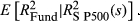
FVX Formulation 1 is first applied using the implied volatility input (No ULPM, Eqn 5). The method is also augmented to incorporate the upper versus lower partial moment (UPLM, Eqn 10). Formulation 2 of the FVX is also fitted in the form  (Eqn 7), along with a similar linear model using CBOE VIX in the form α + β × VIX2 (Eqn 9). In all cases, the methods are fitted using an ever-expanding window of historic data. These methods are compared with more conventional methods including GARCH (1,1) and EWMA, along with trailing historic volatility calculated across all data (HV all) and trailing historic volatility calculated over the previous 22 days (HV 22 day). Some methods could not be fitted for all funds. This group is labelled ‘NA’.
Table 2 shows average results of the regression of realised fund volatility on the fund volatility indices across 14 020 of 14 925 funds for which all methods could be applied. There were 905 funds for which one or more methods could not be applied. Table 3 shows the distribution of adjusted R2 for the regressions. For example, the results of regressing realised volatility on FVX Formulation 1 (ULPM) yielded an adjusted R2 > 0.8 for 254 funds.
| Average intercept | Average slope | Adjusted R2 | |
|---|---|---|---|
| Fund Volatility Index (FVX) Formulation 1: No ULPM | |||

|
1.1359 | 1.0658 | 0.5798 |
| FVX Formulation 1: ULPM | |||
|
1.2918 | 1.0438 | 0.5814 |
| FVX Formulation 2 | |||

|
6.5071 | 0.7069 | 0.5928 |
| Linear model Chicago Board Options Exchange VIX | |||
| α + β × VIX2 | 6.4999 | 0.6996 | 0.5838 |
| Other methods | |||
| Historic volatility—22 day | 6.7149 | 0.6945 | 0.5152 |
| Historic volatility—all data | 3.3721 | 0.9050 | 0.1265 |
| GARCH (1,1) | 10.7225 | 0.5134 | 0.2356 |
| EWMA | 6.1930 | 0.7145 | 0.5562 |
- The table shows results of regressing 22-day realised volatility on the fund volatility indices. The simple average is taken for the intercept, slope and adjusted R2, across the 14 020 funds for which all methods could be applied. Statistical significance is measured using the method of Newey and West (1987, 1994) to account for overlapping observations. Daily return data were available from September 1998 to October 2009. The number of observations varies for different funds.
| Adjusted R2 | Fund Volatility Index (FVX) Formulation 1 | FVX Formulation 2 | Linear Model Chicago Board Options Exchange VIX | Other methods | ||||
|---|---|---|---|---|---|---|---|---|
| No ULPMa | ULPMb |

|
α + β × VIX2 | HV 22 day | HV all | GARCH (1,1) | EWMA | |
| NAc | 736 | 736 | 739 | 739 | 628 | 628 | 762 | 630 |
| <0.1 | 563 | 579 | 625 | 671 | 663 | 8362 | 1796 | 616 |
| 0.1–0.2 | 397 | 362 | 324 | 302 | 518 | 2237 | 3114 | 446 |
| 0.2–0.3 | 447 | 415 | 352 | 393 | 572 | 1987 | 5400 | 525 |
| 0.3–0.4 | 583 | 595 | 543 | 576 | 823 | 977 | 3063 | 662 |
| 0.4–0.5 | 1135 | 1176 | 845 | 838 | 2340 | 347 | 658 | 1166 |
| 0.5–0.6 | 2809 | 2769 | 2049 | 2382 | 4753 | 228 | 103 | 3718 |
| 0.6–0.7 | 5146 | 5139 | 6156 | 6072 | 4154 | 102 | 29 | 5507 |
| 0.7–0.8 | 2870 | 2900 | 3099 | 2770 | 439 | 43 | — | 1626 |
| 0.8–0.9 | 217 | 233 | 192 | 177 | 35 | 14 | — | 27 |
| 0.9–1.0 | 22 | 21 | 1 | 5 | — | — | — | 2 |
| 14 925 | 14 925 | 14 925 | 14 925 | 14 925 | 14 925 | 14 925 | 14 925 | |
- The table shows the results of regressing 22-day realised volatility on the fund volatility indices, across all 14 925 funds. Statistical significance is measured using the method of Newey and West (1987, 1994) to account for overlapping observations. Daily return data were available from September 1998 to October 2009. The number of observations varies for different funds.
- a
- b

- c Method could not be applied.
The results in Tables 2 and 3 demonstrate that FVX Formulations 1 and 2 outperform other methods particularly the GARCH (1,1) model that tends to be overparameterised. The FVX produces a high adjusted R2 against close–close volatility, with lower bias than any of the other methods. The results also highlight the advantage of the generality of Formulation 1 of the FVX. In particular, the upper versus lower partial moment term can be incorporated into the fit, to capture portfolio insurance behaviour amongst funds. In unreported results, the additional term was found to be significant at the 5 percent level for almost all funds across the majority of data.
Table 4 shows the average adjusted R2 results by fund category, demonstrating that the method worked well for all six categories. Consistency in results illustrates that the method is broadly applicable across funds that maintain at least 80 percent exposure to equities.
| Average adjusted R2 | Growth and income | Growth | Capital appreciation | S&P 500 index obj | Small-cap | Mid-cap |
|---|---|---|---|---|---|---|
| Fund Volatility Index (FVX) Formulation 1: No ULPM | ||||||

|
0.5978 | 0.5817 | 0.5449 | 0.6147 | 0.5586 | 0.5741 |
| FVX Formulation 1: ULPM | ||||||
|
0.6001 | 0.5835 | 0.5463 | 0.6181 | 0.5595 | 0.5743 |
| FVX Formulation 2 | ||||||

|
0.6077 | 0.5952 | 0.5652 | 0.6469 | 0.5675 | 0.5923 |
| Linear Model Chicago Board Options Exchange VIX | ||||||
| α + β × VIX2 | 0.5983 | 0.5865 | 0.5554 | 0.6368 | 0.5576 | 0.5845 |
| Other methods | ||||||
| Historic volatility—22 day | 0.5276 | 0.5103 | 0.4737 | 0.5356 | 0.5051 | 0.5306 |
| Historic volatility—all data | 0.1204 | 0.1403 | 0.1327 | 0.0705 | 0.1145 | 0.1198 |
| GARCH (1,1) | 0.2222 | 0.2740 | 0.2310 | 0.3061 | 0.1931 | 0.1946 |
| EWMA | 0.5717 | 0.5512 | 0.5070 | 0.5857 | 0.5398 | 0.5755 |
- The table shows the results of regressing 22-day realised volatility on the fund volatility indices. The simple average is taken for the adjusted R2 across the 14 020 funds for which all methods could be applied. Fund groups are defined in Appendix. Statistical significance is measured using the method of Newey and West (1987, 1994) to account for overlapping observations. Daily return data were available from September 1998 to October 2009. The number of observations varies for different funds.
5 Concluding remarks
All investors could benefit from a regular and reliable predictor of fund volatility. This study develops a measure called the FVX that reflects expectations of fund volatility and can facilitate the pricing of portfolio insurance (Whaley, 2009). The FVX is based in theory and provides a reliable and unbiased estimate of short-term realised market volatility. The methodology has been applied to short-term volatility forecasts, but it is equally applicable to forecasts over longer periods. It can be updated daily or even intraday without requiring up-to-date fund return data. By comparison, existing methods or alternatives based on the VIX are not based in theory. They prove to be unreliable and biased and are more reliant on up-to-date fund data.
The FVX is more general than existing methods. The generality of the FVX makes it an ideal basis for the development of hedging strategies for fund volatility, for example using derivatives such as forward variance swaps and VIX futures. The FVX is flexible enough to capture skewness in the return distribution for some individual funds, through the incorporation of additional terms like the upper versus lower partial moment of fund volatility versus the market. The method can also be extended to projections of higher moments of fund returns, as well as projections of downside and tail risk.
Notes
Appendix A: Summary of mutual fund objective groups
Funds are categorised into different groups based on objective codes available from WRDS. The number of mutual funds in each category is shown. The largest five funds in each group are listed in order according to average funds under management. A total of 14 925 funds were studied in total.
| Funds (No.) | Objective codes | Largest five funds |
|---|---|---|
| Growth and income funds (3795) |
|
|
| Growth funds (5747) |
|
|
| Capital appreciation funds (615) |
|
|
| S&P 500 Index objective funds (293) |
|
|
| Small-cap funds (2592) |
|
|
| Mid-cap funds (1883) |
|
|