MetaPopGen: an r package to simulate population genetics in large size metapopulations
Abstract
Population genetics simulation models are useful tools to study the effects of demography and environmental factors on genetic variation and genetic differentiation. They allow for studying species and populations with complex life histories, spatial distribution and many other complicating factors that make analytical treatment impracticable. Most simulation models are individual-based: this poses a limitation to simulation of very large populations because of the limits in computer memory and long computation times. To overcome these limitations, we propose an intermediate approach that allows modelling of very complex demographic scenarios, which would be intractable with analytical models, and removes the limitations imposed by large population size, which affect individual-based simulation models. We implement this approach in a software package for the r environment, MetaPopGen. The innovative concept of this approach with respect to the other population genetic simulators is that it focuses on genotype numbers rather than on individuals. Genotype numbers are iterated through time by using random number generators for appropriate probabilistic distributions to reproduce the stochasticity inherent to Mendelian segregation, survival, dispersal and reproduction. Features included in the model are age structure, monoecious and dioecious (or separate sexes) life cycles, mutation, dispersal and selection. The model simulates only one locus at a time. All demographic parameters can be genotype-, sex-, age-, deme- and time-dependent. MetaPopGen is therefore indicated to study large populations and very complex demographic scenarios. We illustrate the capabilities of MetaPopGen by applying it to the case of a marine fish metapopulation in the Mediterranean Sea.
Introduction
Simulation models are extremely useful tools to investigate population genetic processes and patterns for evolutionary and conservation applications (Epperson et al. 2010; Hoban et al. 2012). Simulators can be used to predict the effects of complex demography on population structure and genetic variation. They can help to understand how demographic processes and historical events shape the genetic diversity and differentiation of species. In conservation biology, population genetics simulators are particularly useful to study the genetic processes associated with risk of extinction, inbreeding and outbreeding depression, translocations and re-introductions (Hoban 2014). Another purpose of simulators is statistical inference, where simulations are used to infer parameters such as the strength of selection or the duration of bottlenecks (Hoban et al. 2012).
There are many simulation models available. Hoban et al. (2012) thoroughly reviewed 49 different simulation models producing artificial data sets of genetic polymorphisms. The website ‘Genetic Simulation Resources’ (https://popmodels.cancercontrol.cancer.gov/gsr) contains an up-to-date list of the available simulators. The existing population genetics simulation models can account for a variety of life histories, spatial configuration and genetic features. The simplest models simulate populations with discrete, nonoverlapping generations, constant vital rates and simple forms of population subdivision and dispersal [e.g. EasyPop (Balloux 2001)], while more sophisticated models account for spatial subdivision of populations, complex pattern of migration and different types of natural selection [e.g. QuantiNemo (Neuenschwander et al. 2008)].
Some models are population-based in the sense that populations are explicitly identified [e.g. EasyPop (Balloux 2001)]. Each simulated individual belongs to a population and moves (migrates) between populations. In some other models, in particular spatially explicit models [e.g. CDPOP (Landguth & Cushman 2010)], populations are not considered explicitly. Most models are nonetheless individual based in the sense that each individual is simulated as an object characterized by its genotype, age, sex and other life history characteristics. Individuals can move, die, be born, age and grow. Individual-based models offer a very versatile tool and can in theory accommodate any possible evolutionary scenario. In addition, genetic individual-based models correctly account for random biological processes such as demographic stochasticity and random genetic drift. Simulators can be further classified into forward-time and backward-time simulators; the latter ones are based on the coalescent theory and are efficient because they limit the number of simulated individuals. However, backward-time simulators do not allow monitoring changes in the genetic composition of a population by analysing samples at specific time intervals.
Forward-time individual-based models can present limitations on the number of simulated individuals, because of the memory limits of computers and the long computation times required when simulating a large number of objects. This poses a limitation in the utilization of forward-time individual-based models to simulate the genetics of very large populations, with hundreds of thousands or millions of individuals. Yet, such populations are very common in nature: for example, a single adult female of the European eel (Anguilla anguilla) can produce several millions of eggs (MacNamara & McCarthy 2012); plant populations consist of thousands of potentially interacting individuals. In these cases, forward-time individual-based models can easily become impractical because they cannot simulate large number of individuals in reasonable time or simply because the amount of computer memory required to store such a large number of object is prohibitive.
An alternative to forward-time individual-based simulation models is analytical models, where explicit equations are used to link together genetic quantities of interests analytically. The population genetics literature offers many of such type of models. Analytical models present an enormous variety in complexity accounting to factors ranging from, for example, the relationship between migration rate and allele frequency change in the continental-island model (Hedrick 1985) to models taking into account stochastic processes and several processes altogether. The most complex analytical models can account for stochastic processes, population subdivision, migration, mutation and a variety of life history characteristics such as separate sexes and overlapping generations (Charlesworth 1994; Rousset 2004). However, as complex as they are, analytical models present limitations to the complexity of the demographic and genetic scenarios that can be represented and solved. Indeed, moderately complex biological scenarios (such as populations with overlapping generations and spatial subdivision) quickly become extremely complex mathematical models that are difficult or even impossible to solve using analytical techniques. For this reason, some analytical models can only be solved using approximations (for example, the diffusion approximation) and simplifications. Therefore, while forward-time simulation models can virtually accommodate very complex scenarios and are limited by computing time and capabilities, analytical models are limited in the complexity of scenarios that can be represented by individual-based simulation.
To overcome the difficulties presented by forward-time simulation and analytical models, we propose to use an intermediate approach that allows modelling of very complex demographic scenarios, which would be intractable using only analytical models, and removes the limitations imposed by large population size, which would affect a purely forward-time individual-based model. In the simulation model presented in this study, MetaPopGen, the number of individuals is not a limiting factor. This is possible because the individual-based approach is abandoned in favour of a probabilistic approach that accounts for random processes such as Mendelian segregation and demographic stochasticity. More precisely, random number generators for appropriate probabilistic distributions are used to mimic the stochasticity inherent to these processes. MetaPopGen is therefore adapted to simulate large size populations, or combinations of large and small size populations. Features included in the model are age structure, monoecious and dioecious (or separate sexes) life cycles, mutation, dispersal and selection. In addition, all demographic parameters can be genotype-, sex-, age-, deme- and time-dependent, thus making MetaPopGen very powerful with respect to the variety of demographic scenarios that can be simulated. The major limitation of MetaPopGen is the possibility of simulating only one locus at a time. The reasons underlying this limitation will be presented in the discussion.
The innovative concept of MetaPopGen with respect to the other population genetic simulators is that it focuses on genotypes and allele numbers rather than on individuals. This makes MetaPopGen useful for predictive studies such as investigating the statistical properties of genotype frequencies in time and their link to demographic and biological processes. Genotype frequencies are widely used to measure genetic diversity and genetic differentiation, two quantities of great interest to describe genetic biodiversity and elaborate genetic conservation plans. Therefore, focusing on the absolute numbers or on the relative frequencies of types of individuals (geno-types) makes it possible to capture the most important variables to study population genetics and evolution.
Simulating genotype numbers rather than individual genotypes allows overcoming the limitations imposed by computer memory to the number of simulated objects. In MetaPopGen, the number of individuals of a certain genotype is iterated through time and undergoes changes due to mortality, dispersal and reproduction. At the end of the simulation, the status of the metapopulation is fully described by the number of individuals of each genotype in each deme, sex, age class and time. MetaPopGen also includes functions to calculate the allele frequencies and basic population genetics parameters such as FST.
In the following, we describe the simulation model and the input parameters. We give a brief description of the inner functions that simulate biological processes, and we exemplify the usefulness of MetaPopGen by applying it to a simple idealized metapopulation and to a case study of marine metapopulations.
The simulation model
MetaPopGen is implemented in a package for the r environment (R Development Core Team 2011). It permits to simulate a population structured into n demes, with z age classes, either monoecious or dioecious, and connected by dispersal. We describe here the monoecious model. The user defines the demographic and genetic parameters and the initial genetic composition of the population. Nijxt is the number of individuals of genotype j (1 < j < m), age x (1 < x < z), in deme i (1 < i < n) at time t (1 < t < tmax). The maximum age z, the number of demes n, the number of simulated time steps tmax and the maximum number of possible genotypes m [given by the number of alleles l: m = l(l + 1)/2] are set by the user. The user also enters the initial composition of the population Nijx1, i.e. the number of individuals of each genotype, for all demes and ages at time t = 1.
Then, the simulator iterates Nijxt, the number of possible genotypes through time, by using the functions describing survival, reproduction, dispersal and recruitment and the demographic and genetic parameters (survival probabilities, fecundities, mutation probabilities, dispersal probabilities, juvenile carrying capacity) defined by the user.
The output of the simulation is the variable Nijxt at each time step. This variable can be used to calculate various indices of genetic diversity and differentiation, such as allele frequencies and FST. In the following, we describe the demographic and genetic parameters used by the simulator and the principles underlying model functioning.
Demographic and genetic parameters
The parameters used for the simulations are (i) the age-, deme-, genotype- and time-specific survival probabilities σijxt (where i is deme, j is genotype, x is age and t is time); (ii) the age-, deme-, genotype- and time-specific male and female fecundities, ϕMijxt and ϕFijxt; (iii) the time-specific dispersal probabilities δirt (from deme r to deme i); (iv) the mutation probability μuv (from allele v to allele u); and (v) the deme- and time-specific juvenile carrying capacity K0it. These parameters must be defined by the user. The female fecundity is the number of per capita produced embryo sacs (for plants) or eggs (for animals). The male fecundity is the number of per capita produced pollen grains (for plants) or sperms (for animals). Fecundities are usually large numbers, but this is not a limit for the simulator. Therefore, it is possible to simulate species with very large female fecundities, such as trees or fishes, and to use very large numbers for male fecundities, which are usually very large and often unknown.
where W is the absolute fitness of the A2A2 genotype, s is the selection coefficient and h is the heterozygous effect; this is the usual notation for models with selection (Hedrick 1985). In this case, there is selection against the A1 allele. Using a selection coefficient s = 1 and a heterozygous effect h = 0.7 and considering that only survival rates are affected by selection, fitness can be equated to survival probability. This will give a survival probability σijxt = 0 for genotype j = A1A1 and σijxt = 0.3·σiuxt for genotypes j = A1A2 and u = A2A2, i.e. the survival probability of the A1A2 heterozygote is 30% that of the A2A2 homozygote.
The dispersal probabilities δirt are the probabilities that a newborn in deme r will successfully disperse to deme i at time t. It is possible to define arbitrarily complex and time-varying dispersal probabilities. This is useful when empirical estimates of dispersal probabilities are available, for example from mark–recapture studies or genetic assignment tests, or also from biophysical simulations in marine ecosystem, as in the example application below.
The possibility of defining temporally variable survival, fecundity and dispersal parameters allows for modelling environmental stochasticity, changing environmental conditions, climate change, temporally varying selection, etc. This is an important application of the method.
The mutation probabilities μuv are the probabilities that a gamete of type (allele) v will mutate to type u. The mutation model used here for genetics is a ‘K-allele model’, i.e. the number of alleles is constant and equal to the user-defined parameter l.
The juvenile carrying capacity, K0it, is a parameter used in the density-dependent recruitment function and is the maximum number of juvenile individuals that can recruit to each deme each time step. Density-dependent recruitment is useful to prevent the simulated population from growing without bound.
Model functioning
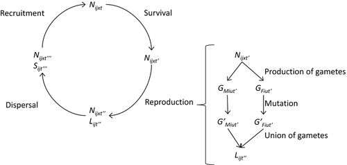
The modelled life cycle consists of four consecutive phases: survival, reproduction, dispersal and recruitment (Fig. 1). The reproductive phase is subdivided into three subphases: production of gametes, mutation and union of gametes. Each phase or subphase is modelled using the probabilistic functions described hereafter. t indicates time before survival; t’ indicates time after survival and before reproduction; t’’ indicates time after reproduction and before dispersal; t’’’ indicates time after dispersal and before recruitment.
Survival phase
Reproduction phase
The reproduction phase consists of three subphases (Fig. 1): production of gametes, mutation and union of gametes.
Production of gametes
In each deme, the number of gametes produced by a single individual is a Poisson random variable with mean equal to the age-specific fecundity. The total numbers of male and female gametes of type (allele) u in deme i at time t’ are denoted as GMiut’ and GFiut’, respectively. Homozygous individuals produce gametes of only one type. Heterozygous individuals produce two types of gametes according to a binomial distribution with probability 0.5 (Mendelian segregation).
Mutation
Union of gametes
where MULTIHYPER indicates the random number generator for the multivariate hypergeometric distribution (the rMWNCHypergeo function in the r package BiasedUrn) with parameters G’Fiut’ (number of sampled gametes: number of female gametes of type u = A1) and G’Miut’ (initial vector of number of gametes: number of male gametes of each type); Li•t’’ is the number of newborns of each genotype and • = [A1A1, A1A2, A1A3]. The multivariate hypergeometric random number generator is repeated for each allele u to obtain the total number of newborns of each genotype. If the number of male gametes is smaller than the number of female gametes, the function is the same but the female and male variables are exchanged.
With very large numbers of gametes, the multivariate hypergeometric distribution approaches the multinomial distribution. In most cases, the multinomial approximation would be adequate. However, the hypergeometric random number generator correctly accounts for sampling effects in the union of gametes process. While this sampling effect is likely to be small when the number of gametes is large, it contributes to random genetic drift when the number of female and/or male gametes is very small.
Dispersal phase
where δ•it is the probability vector (probability of dispersal from deme i to the other demes) and Lijt’’ is the number of trials (number of newborns in deme i of genotype j). The drawing is repeated over genotypes and demes of origin to find the final number of juveniles in each deme and of each genotype Sijt’’’.
Recruitment phase
That is, as the total number of juveniles Sijt’’’ in the deme i increases, the survival of juveniles decreases to zero and the number of recruits tends asymptotically to K0it, the maximum total recruitment in the deme at that time.
Applications
Island model
We compared the results of MetaPopGen with those obtained using Nemo 2.2.0, a similar forward-time individual-based simulator (Guillaume & Rougemont 2006). The r script and the Nemo ini files used to perform these simulations are available as online supporting information.
The theoretical prediction for the island model from the relationship FST ≈ 1/(1 + 4·Ne·m), where Ne is the size of each deme (hence Ne = 3000) and m the migration rate among demes (m = 0.1), is FST ≈ 0.00083. The genetic differentiation index calculated with MetaPopGen stabilized after about 50 generations at FST = 0.00062 ± 0.0002 (mean ± standard deviation), very close to the theoretical expectation. Nemo gave a statistically equal result, FST = 0.00065 ± 0.0002. The agreement between the results of Nemo and MetaPopGen confirms the equivalence of the individual-based approach with the approach of MetaPopGen based on random number generators. The computation times for MetaPopGen and Nemo were about 8 s and 52 s per replicate, respectively, on the same laptop computer (T5500 intel core2 duo Processor; 1.66 GHz; 1 Gb RAM).
A marine metapopulation
We further illustrate the capabilities of MetaPopGen by simulating metapopulation genetics in the system of marine protected areas (MPAs) of the Mediterranean Sea [Fig. 2; (Andrello et al. 2013)]. The data set and the code used for simulations and analyses are available as online supporting information. Due to their small size and the large distances between them, each of the 115 Mediterranean MPAs can be considered as a single deme. In reality, most marine species in the Mediterranean Sea are distributed continuously over the continental shelf and are present also outside the boundaries of MPAs. Here, we consider the case of a hypothetical species that can survive only inside MPAs’ boundaries, for example because fishing outside protected areas is too intense to allow the species to persist. The dusky grouper Epinephelus marginatus (Lowe 1834) has higher abundances in well-protected and well-enforced MPAs than in nearby fished areas (Garcia-Charton et al. 2004; Guidetti & Sala 2007), is sedentary in the adult phase and has mobile larvae; thus, it can be considered as an example of such a scenario. The simulations were inspired by the biology of this species, but they could not be parameterized to reproduce exactly its life cycle, because many parameters are unknown.
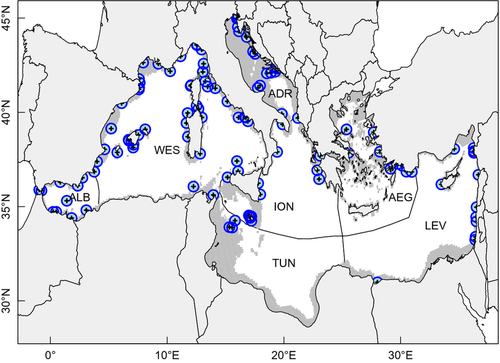
The maximum total recruitment was set to K0it = 1000 in all demes at all times. Sexes were separate, and the number of age classes was set to five. We set time-, genotype-, deme- and age-invariant survival probabilities σFijxt and σMijxt = 0.8 for all i, j, x and t; time-, genotype- and deme-invariant but age-specific fecundities: ϕMijxt = 0 for x < 3 and ϕMijxt = 106 for 3 ≤ x ≤ 5; ϕFijxt = 0 for x < 3 and ϕFijxt = 2·105 for 3 ≤ x ≤ 5. We simulate one locus with two alleles with mutation rates μuv = 10−6 for u ≠ v. The initial number of individuals was drawn from a uniform distribution defined between 0 and 300 for each genotype in each age class for each of the two sexes in each deme. We iterated the simulation for 200 time steps, and we ran 30 replicates of this scenario to evaluate variation among simulations.
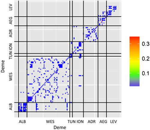
For sessile marine organisms, dispersal among demes is assured by larvae. Larval dispersal probabilities among demes were estimated using a biophysical model of larval dispersal as described in Andrello et al. (2013) to estimate larval dispersal in E. marginatus. The estimations of this previous study allow us to define time-invariant dispersal probabilities δirt's (Fig. 3).
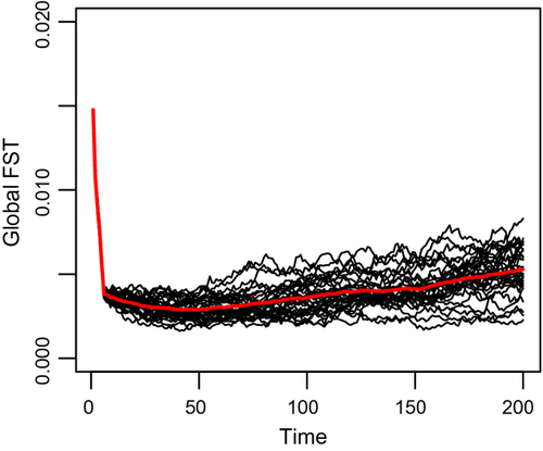
The outcome of the simulations is the number of individuals in each deme at each time step for each sex, genotype and age-class, NMijxt and NFijxt. We calculated the index of genetic differentiation FST among all demes (using the fst.global.dioecious function in MetaPopGen) for each of the 200 time steps of simulation (Fig. 4). The initial global differentiation due to the initial random distribution of genotypes (FST ≈ 0.015) decreased quickly under the effects of dispersal. Then, the genetic differentiation among demes started increasing as a result of genetic drift and reached the value FST ≈ 0.0053 at the end of the simulation. This value is similar to the empirical estimates of FST obtained for the dusky grouper [FST = 0.01 (Schunter et al. 2011)]. FST increased at a steady annual rate of 1.1·10−5 and varied among the 30 replicates. The variance of FST among replicates was 0 at the beginning of the simulation, because all replicates started with the same distribution of individuals over genotypes, ages and demes (same NMijx1 and NFijx1 for all replicates) and increased with time at an annual rate of 8.9·10−9 (linear regression, adj-R2 = 0.92, P < 10−15).
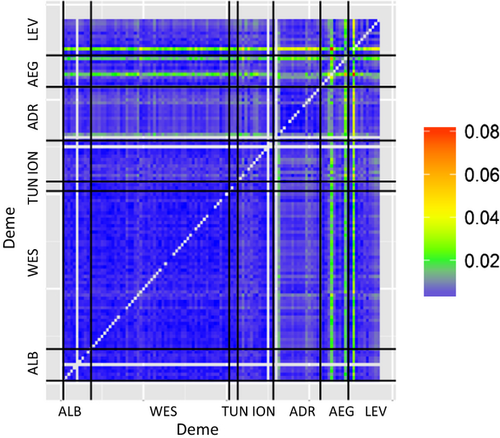
We then tested whether genetic differentiation increased as the distance between demes increases (isolation by distance) or as the dispersal probability between sites decreased. In this application, pairwise FST increased with spatial distance, but not significantly (Mantel test: z-statistic = 35479, P = 0.084, 9999 permutations). FST decreased significantly with dispersal probability (Mantel test: z-statistic = 0.00034, P = 0.0001, 9999 permutations). In this case, the highly significant relationship between pairwise FST and dispersal probability shows that genetic differentiation is explained more strongly by dispersal probability than by spatial distance.
Discussion
In this article, we have described a new population genetics simulation model, MetaPopGen, an r package to simulate population genetics in very large metapopulations. There are two features of MetaPopGen that appear as strong novel points relative to the existing population genetics simulation models available today: (i) the ability to simulate demes and metapopulations with very large size and (ii) the possibility of using temporally variable demographic parameters (although this possibility is already included in some models).
The ability of simulating very large population sizes makes MetaPopGen a very useful tool to study populations of very fecund organisms, such as plants and fish, and to study large populations. Up to now, simulating genetics in very large populations was prohibitive because of computing time and memory. The only alternative to simulation is analytical models, but often these are limited in the complexity of life history and population structures that can be treated. Simplifications to analytical models can be made by neglecting random processes so that the models become deterministic and are much simpler and easier to solve. As large populations do not undergo strong levels of genetic drift, such stochastic processes can safely be neglected in many cases, and therefore, there is no need to use simulation models. Another approach is using individual-based models that simplify the life cycle phases with high abundance that are therefore less affected by genetic drift (e.g. Nemo implements backward migration probabilities to simulate migration when demes are at carrying capacity; Guillaume & Rougemont 2006). However, natural populations often consist of collections of large and small demes and studying this collection as a system of connected demes exchanging migrants requires consideration of the genetic drift experienced by the smaller demes. This is not possible by using analytical models that are not stochastic. MetaPopGen allows for variable deme sizes and is therefore suitable for such systems. To our knowledge, MetaPopGen is the first population genetics simulation model that is not limited by the number of individuals in the simulated demes, thanks to the focus on genotype numbers rather than individuals and the use of probabilistic distribution to simulate the evolution of genotype numbers through time.
There are a few population genetics simulator capable of taking into account variable demographic parameters [e.g. rmetasim (Strand 2002), SimuPop (Peng & Kimmel 2005) and QuantiNemo (Neuenschwander et al. 2008)]. MetaPopGen is extremely versatile on the temporal variation in demographic parameters because the choice of demographic parameters for each time step is left to the user. This permits to simulate a wide variety of scenarios, including environmental stochasticity, where survival and fecundity changes randomly through time; or scenarios of directional environmental change, where vital rates change steadily through time as a result of a long-term trend, such as climate change; or combination of these two processes. It is also possible to simulate deme extinction, by setting vital rates to zero or to very low values at a certain time and recolonization. An option exists for defining vital rates in a data frame format so that it is possible to use a spreadsheet to format the data and then import them into the r environment.
The major limitation of MetaPopGen is the simulation of only one locus at a time. While a multilocus version of the programme would be possible technically, we decided to not pursue this development. The reason is that simulating more than one locus would imply increasing the number of possible multilocus genotypes that the simulator has to keep track of, and the number of possible genotypes increases geometrically with the number of loci. For example, consider the case of a locus with 10 alleles. Simulating such a locus implies keeping track of 55 genotypes (the number of possible genotypes at a locus is m = k(k + 1)/2, where k is the number of alleles), and this is well within the capabilities of the simulator. Simulating two such loci would imply keeping track of 552 = 3025 possible genotypes; it becomes apparent than increasing the number of loci would quickly overflow the memory capacity of even the most modern computer. A similar limitation applies to the number of possible demes and age classes, as increasing these would increase the size of the multidimensional arrays that store the genetic information, although not geometrically as in the case of multilocus genotypes; in addition, MetaPopGen offers a way to overcome the limitation on the number of demes and age classes by reducing information storage in some cases (e.g. with time-invariant parameters and by storing on disc the results of some iterations only). These limitations parallel the limitation on the number of individuals in individual-based simulators.
The strengths and weaknesses of MetaPopGen with respect to other forward-time simulators suggest which simulator can be used depending on the evolutionary scenario. While individual-based simulators are well adapted to multilocus systems where the number of individuals is not too large, MetaPopGen is adapted to simulate scenarios with large numbers of individuals but only one locus. The optimal forward-time simulator capable of dealing with multilocus populations of very large size probably does not exist, and the correct practice is to choose the most adapted simulator to the situation of interest. Therefore, MetaPopGen is not made for multilocus system, such as hundreds of thousand single nucleotide polymorphisms system. If the purpose is to create artificial data sets of multilocus genotypes, we recommend the use of individual-based simulators. Conversely, we encourage using MetaPopGen to predict the effects of complex demographic scenarios on population genetic structure and diversity. If needed, one can derive multilocus expectations of genetic variables (genotype frequencies, allele frequencies, FST…) by repeating several times the simulation with the same set of demographic parameters, as we did in the marine metapopulation example above (e.g. Fig. 4). If the loci are independent, this procedure works well. Simulating linked loci is more challenging, and the best option for this is still using an individual-based simulator.
A classification using the criteria developed by Hoban et al. (2012), their Table III) would place MetaPopGen among the most complex simulators. These criteria concern five aspects of the scenarios that the simulator can model: life history, demography, selection, migration and recombination. MetaPopGen can accommodate for complex life histories with overlapping generations, age- and deme-specific survival and fecundities. The demography is complex because time-varying parameters can be set for survival, fecundity and dispersal. Selection is complex, because it can be deme- and time-dependent, although no epistasis- or frequency-dependent selection can be simulated. Migration is basic, because based on user-defined matrices, but the matrices can be temporally dependent. Finally, there is no recombination because only one locus is simulated. Pedagog (Coombs et al. 2010) and rmetasim (Strand 2002) are the most similar simulators to MetaPopGen.
We presented a simple example to illustrate the functioning of MetaPopGen. A system of 115 demes (corresponding to Mediterranean MPAs) was simulated using a dispersal matrix estimated through biophysical simulations. We assessed the stochasticity of the simulations by running many replicates of the same scenario. This allowed us to estimate not only a single value of the genetic differentiation index FST but also a distribution, which can be compared to empirical values obtained through the analysis of molecular markers.
In conclusion, MetaPopGen is a very powerful and fast simulator capable of modelling arbitrarily complex life history and demographic scenarios for prediction purposes. Even, if in the example above we used the same demographic parameters for all genotypes, demes and times, MetaPopGen can accept time-, deme- and genotype-dependent parameters and is very useful to explore scenarios for which an analytical treatment is challenging. With the increasing accumulation of demographic and dispersal data on a variety of species, understanding the effects of complex demography on population structure and genetic variation will be possible via simulation and MetaPopGen offers the possibility to do so.
Acknowledgements
We thank Sean Hoban and three anonymous reviewers for comments on a previous version of this manuscript. This work was funded by ‘Fondation pour la Recherche sur la Biodiversité’ (www.fondationbiodiversite.fr) and ‘Fondation Total’ (fondation.total.com) through the ‘Fishconnect’ project.
References
M.A. developed and programmed MetaPopGen; both authors conceived the ideas and wrote the manuscript.
Data Accessibility
The r script and the Nemo ini file for the simulation of the island model and the r scripts and RData files for the simulation of the Mediterranean metapopulation model are available as supporting information.
The MetaPopGen r package can be downloaded from: https://sites.google.com/site/marcoandrello/metapopgen.


