Topographic elastic least-squares reverse time migration based on vector P- and S-wave equations in the curvilinear coordinates
ABSTRACT
Elastic least-squares reverse time migration has been applied to multi-component seismic data to obtain high-quality images. However, the final images may suffer from artefacts caused by P- and S-wave crosstalk and severe spurious diffractions caused by complex topographic surface conditions. To suppress these crosstalk artefacts and spurious diffractions, we have developed a topographic separated-wavefield elastic least-squares reverse time migration algorithm. In this method, we apply P- and S-wave separated elastic velocity–stress wave equations in the curvilinear coordinates to derive demigration equations and gradient formulas with respect to P- and S-velocity. For the implementation of topographic separated-wavefield elastic least-squares reverse time migration, the wavefields, gradient directions and step lengths are all calculated in the curvilinear coordinates. Numerical experiments conducted with the two-component data synthetized by a three-topographic-layer with anomalies model and the Canadian Foothills model are considered to verify our method. The results reveal that compared with the conventional method, our method promises imaging results with higher resolution and has a faster residual convergence speed. Finally, we carry out numerical examples on noisy data, imperfect migration velocity and inaccurate surface elevation to analyse its sensitivity to noise, migration velocity and surface elevation error. The results prove that our method is less sensitive to noise compared with the conventional elastic least-squares reverse time migration and needs good migration velocities as other least-squares reverse time migration methods. In addition, when implementing the proposed method, an accurate surface elevation should be obtained by global positioning system to yield high-quality images.
INTRODUCTION
The conventional reverse time migration (RTM) method tends to produce low-resolution and signal-noise ratio images with unbalanced amplitude, since it uses an adjoint of the modelling operator rather than its inverse (Claerbout 1992; Kuehl and Sacchi 1999; Nemeth, Wu and Schuster 1999; Duquet, Marfurt and Dellinger 2000; Etgen, Gray and Zhang 2009). In contrast, least-squares migration (LSM) can produce high-quality images with more balanced amplitudes, fewer artefacts and higher resolution (Nemeth Wu and Schuster 1999; Duquet, Marfurt and Dellinger 2000; Ronen and Liner 2000; Fomel et al. 2002). Moreover, LSM implemented with RTM is called ‘least-squares reverse time migration (LSRTM)’, which can reduce artefacts in the standard RTM image in addition to suppress data acquisition footprint.
However, complex topographic surface conditions always pose serious troubles when trying to obtain seismic images. To overcome the problem, some instructive studies implementing finite-difference (FD) methods (Virieux 1986), finite-element methods (Moczo et al. 1997), pseudo-spectral methods (Fornberg 1988), spectral element methods (Komatitsch and Tromp 2002) have been developed for calculating topographic seismic wavefields. FD methods have been widely used due to their small memory storage, high computational efficiency, robustness and easy implementation (Levander 1988). The conventional FD methods generally discretize the computational model into uniform rectangular grids, leading to the challenging problem of modelling seismic wave propagation in media with extreme surface topography. One effort to overcome this problem of the uniform rectangular grids in the conventional FD method is using non-uniform grids, such as curvilinear grids (Fornberg 1988; Tessmer, Kosloff and Behle 1992; Tessmer and Kosloff 1994; Hestholm and Ruud 1994; Nielsen, Berg and Skovgaard 1994; Qu et al. 2017a,b, 2018a), variable grids (Moczo 1989; Jastram and Tessemer 1994) and unstructured grids (Kaser and Igel 2001).
The computational requirement for LSM is very demanding; hence, some methods have been proposed to overcome this issue. For example, a deblurring filter is applied as a pre-conditioner to LSM, which results in one-third cost of conventional LSM and meanwhile produces an acceptable migration image (Aoki and Schuster 2009). Least-squares slip-step migration based on double square root equation is applied to speed up the convergence speed (Kuehl and Sacchi 1999, 2001, 2003). Encoding multisource LSRTM is employed to reduce computational cost to a level comparable to RTM by blending many shot gathers together to form one supergather and suppress the crosstalk noise between different shots by applying the encoding functions (Dai, Wang and Schuster 2011; Dai, Fowler and Schuster 2012; Huang and Schuster 2012; Dai, Huang and Schuster 2013; Dai and Schuster 2013).
Besides the computational efficiency, LSRTM has some difficulties in producing good images when applied to field data because of its linear assumptions and inaccurate migration velocity model. A non-linear LSRTM is proposed to overcome the shortness of the linear approximation, which calculates the synthetic data directly by using the reflectivity rather than assuming linearity (Yao and Jakubowicz 2012). Tan and Huang (2014) applied a wavefield-separation imaging condition into LSRTM, which separates the wavefields into upgoing, downgoing, leftgoing and rightgoing components, to reduce low-frequency noise and improve steeply dipping structure imaging. Extended Born modelling operator and asymptotic inverse operator are also proposed to speed up the convergence of LSRTM even with an inaccurate migration velocity model (Hou and Symes 2015). In addition, different regularization or pre-conditioning operators are also constructed with LSM to obtain higher-resolution images (Wang and Sacchi 2007; Anagaw and Sacchi 2012; Xue et al. 2016).
Recently, elastic LSRTM (ELSRTM) is developed to obtain P-velocity (vp), S-velocity (vs) (Feng and Schuster 2017) and density (Qu et al. 2018b) perturbation images. Compared with the acoustic LSRTM method, ELSRTM produces fewer artefacts and better resolution images. However, ELSRTM produces multi-component images with P- and S-wave crosstalk artefacts. A separated-wavefield ELSRTM (SELSRTM) method is proposed to enhance imaging quality (Gu, Li and Han 2018). However, the multi-component data need to be separated P- and S-wave data, which serve as the input when implementing the SELSRTM. In this paper, we propose a new topographic SELSRTM (T-SELSRTM) method based on vector P- and S-wave equations in the curvilinear coordinates. In the proposed method, the input observed shot records are the conventional multi-component data dobs (dobsx, dobsz) without implementing wavefield separation.
In this paper, we first briefly describe the theory of conventional LSRTM based on the conjugate gradient method. Then we introduce curvilinear grid generation and coordinates transformation. Thirdly, we implement T-SELSRTM by deriving P- and S-wave separated demigration equation and gradient formula in curvilinear coordinates and provide the computational flow of the proposed T-SELSRTM method. In the numerical examples, we present a three-topographic-layer with anomalies model and a Canadian Foothills model to prove the capability of our T-SELSRTM for vp and vs perturbation imaging. Lastly, we discuss the sensitivity of the proposed T-SELSRTM method to random noise, imperfect migration velocity and inaccurate surface elevation.
THEORY OF LEAST-SQUARES REVERSE TIME MIGRATION
 (1)
(1) , where L denotes the modelling operator and m is the reflectivity model. In this paper, we use the pre-conditioned conjugate gradient (Dai, Fowler and Schuster 2012) method to solve the least-squares inverse problem. The conjugate gradient method uses the following equation to update the reflectivity model:
 (2)
(2) and
and  are the conjugate gradient direction and the step length for the kth iterative step, which are calculated by
 (3)
(3) (4)
(4) (5)
(5) (6)
(6) is the gradient direction for the kth iterative step from the steepest descent method, and
  denotes the corresponding step length; T denotes the transpose of matrices; LT denotes the reverse time migration operator; C is a pre-conditioned operator. In this paper, we introduce the amplitude-preserving migration weights method as the pre-conditioner (Plessix and Mulder 2004). The pre-conditioner approximates the inverse of the Hessian of the least-squares functional, which is difficult to obtain directly.
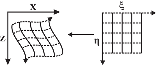
Curvilinear grid generation and coordinates transformation
 (7)
(7)
 ,
,  ,
,  and
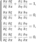
and  to transform the first-order velocity–stress wave equation in the Cartesian system to the curvilinear coordinates, which can be derived from
 (8)
(8)The staggered grid (SG) method is widely used because of its increased stability and ability to suppress numerical dispersion compared with the collocated grid method. Figure 2(a) shows the schematic diagram of standard staggered-grid (SSG) scheme, where the normal stresses (τxx and τzz) are defined in the main grid points, and the velocities (vx and vz) and the shear stress (τxz) are defined in the half grid points.
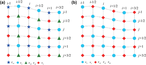
However, when solving the wave equations in the transitional coordinates, some variables need to be calculated by the interpolation method, resulting in error and instability. In this paper, we use the full staggered-grid (FSG) scheme to overcome the error resultant from interpolating (Lebedev 1964). The way to define the grid is shown in Fig. 2(b).
VECTOR P- AND S-WAVE EQUATIONS IN THE CURVILINEAR COORDINATES
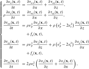 (10)
(10)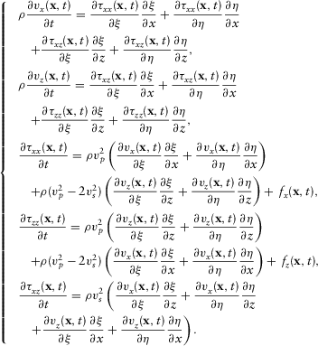 (11)
(11) is curl-free field and S-wave wavefield
  is divergence-free field, we can obtain the following equations:
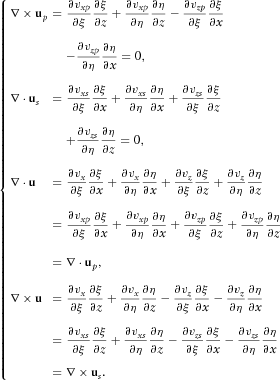 (12)
(12) (13a)
(13a)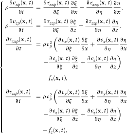 (13b)
(13b)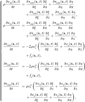 (13c)
(13c)TOPOGRAPHIC ELASTIC DEMIGRATION OPERATOR AND GRADIENT FORMULAS BASED ON WAVEFIELD SEPARATION
 (14)
(14)For simplicity, we make the assumption that the density is accurate with no perturbation. This means that  . Therefore, the density has no effects on the crosstalk between the P- and S-wave images.
Firstly, we formulate the Born approximation P-wave equation. Based on the Born approximation theory, perturbations of velocities will lead to perturbation of wavefields.
 ,
, ,
, ,
,  ,
,  ,
,  ,
,  ,
,  and
and  ) can be separated into background wavefields U0 and perturbation wavefields
  . The relationships between the background and the perturbation wavefields are given by
 (15)
(15)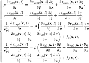 (16)
(16) and ignore the high-order terms to obtain
 (17)
(17)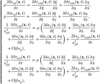 (18)
(18) denotes the high-order term of
  . The P-wave reflectivity model associated with vp perturbation is defined by
 (19)
(19)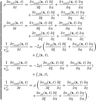 (21)
(21)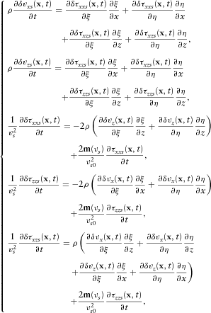 (22)
(22) (23)
(23) and
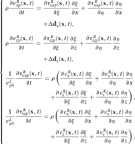
and  as the synthetic shot records in horizontal- and vertical-component, respectively, we have
 (24)
(24) (25)
(25) and
and  denote the difference between synthetic data and observed data in the horizontal and vertical directions, which are given by
 (26)
(26) and
and  are the observed data in the horizontal and vertical components, respectively. When k = 1, in equation 2,
  and in equation 26,
  . Then, equation 2 is changed to
 (27)
(27) and
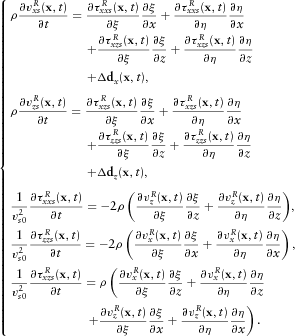
and  are the imaging condition and the gradient direction of vp for the first iteration, respectively. Similarly, we give the S-wave migration equation in curvilinear coordinates as follows:
 (28)
(28) is
is
 (29)
(29) and
and  are the imaging condition and the gradient direction of vs for the first iteration, respectively.
  and
and  will be derived in the following paragraphs. In the proposed T-SELSRTM, we define that
  ,
,  ,
,  and
and  .
. (30)
(30) can be obtained by
 (31)
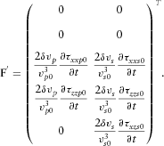
(31) , where L denotes the Born forward modelling operator based on wavefield separation and
  is a new constructed source matrix used to produce wavefields perturbation
  and is written as
 (32)
(32)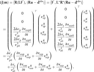 (33)
(33) and
and  , the gradient values for P- and S-wave components, respectively, as follows:
 (34)
(34) (35)
(35) and
and  are the gradient values for P- and S-wave components, respectively. The step length can be calculated as follows:
 (36)
(36) (37)
(37) and
and  are the step length for P- and S-wave components, respectively. The revised conjugate gradient directions and the corresponding steps can be calculated by using equations 5 and 6.
-
Input migration velocity models (vp, vs) in the curvilinear coordinates and observed data dobs (dobsx, dobsz);
-
Mesh the velocity models into curvilinear grids according to the irregular surface and complex underground structures;
-
Transform the velocity models into the curvilinear coordinates;
-
Calculate forward-propagating P-wavefields (τxxp, τzzp) and S-wavefields (τxxs, τzzs, τxzs) in the curvilinear coordinates using equation (13);
-
Calculate back-propagating P-wavefields (
 ) and S-wavefields (
 ,
,  ,
,  ) in the same curvilinear coordinates using equations 25 and 28;
 -
Apply equations 27 and 29 to obtain the image m (mvp, mvs) in the curvilinear coordinates;
-
Calculate scattering wavefields and synthetic shot records dcal (dcalx, dcalz), and obtain the data residual
 ;
; -
If
 (ε can be obtained through the experience in weighing accuracy and calculation. For example, ε = 0.1) or the iteration number reaches a predetermined number of times, transform the images to the Cartesian coordinates and outputting the images; otherwise, calculate back-propagating residual P- and S-wavefields (equations 25 and 28);
 -
Calculate conjugate gradient direction gc (gcvp, gcvs) and step length β (βvp, βvs);
-
Update images m (mvp, mvs);
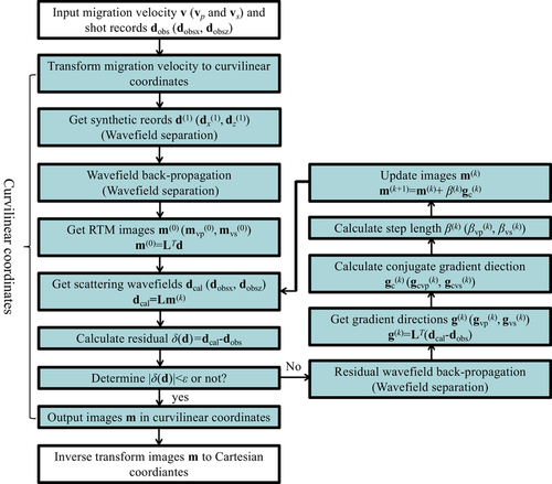
Note that the wavefields, gradient directions and step lengths are all calculated in the curvilinear coordinates and other steps are realized in the Cartesian coordinates. The input observed data are the conventional multi-component records dobs (dobsx, dobsz) with no need of wavefield separation as the pre-processing step. And then the residual P- and S-wavefields are separated during the back-propagation by the separated P- and S-wave migration equation (equations 25 and 28). We track the residuals using the L2 norm of mixed data residuals (dobs) as the conventional ELSRTM.
NUMERICAL EXAMPLES
In this section, we use a three-topographic-layer with an anomalies model and a Canadian Foothills model to test the proposed P- and S-wavefield separated Born forward modelling operator in curvilinear coordinates and T-SELSRTM method. All our simulations are implemented using a time-domain FD method algorithm with the second-order accuracy in time domain and tenth-order accuracy in spatial domain. A complex frequency-shifted perfectly matched layer (CFS-PML) boundary condition (Köhn et al. 2012) is implemented to suppress artificial boundary reflections.
Example 1: Three-topographic-layer with anomalies model
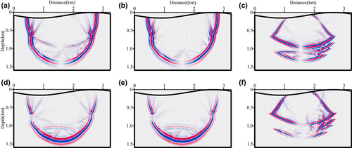
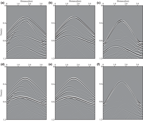
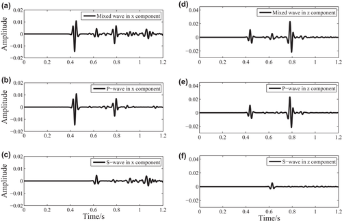
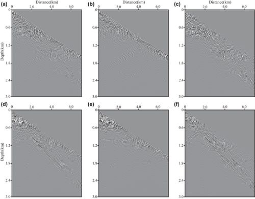
A simple three-topographic-layer with anomalies model in the Cartesian coordinates of 3200 metre x-extent and 1600 metre z-extent (shown in Fig. 4) is used to test the behaviour of our P- and S-wave separated Born modelling (equations 20 and 22). The model is discretized with 400 × 200 gridpoints in the x- and z-directions with a grid spacing of 8 metres. To compare the influence of P- and S-wave, we add a P- and S-velocity anomaly on the left and right of a three-layer model, respectively. The density model is calculated by ρ = 0.23vp0.25 (Gardner et al. 1974). Based on curvilinear grids (Fig. 5), the sag topographic model can be changed to a flat-layered model in curvilinear coordinates (Fig. 6). A Ricker wavelet explosive source with the dominant frequency of 25 Hz is located at (1600 metres, 8 metres). The total record length is 1.2 seconds, and the time sample increment is determined to be 0.6 milliseconds to ensure the numerical calculation stability. The shot is recorded with 401 receivers and 8-minute interval. The reflectivity of the three-topographic-layered with anomalies model in the curvilinear coordinates is given in Fig. 7. The snapshots in the Cartesian coordinates at 390 millisecond propagation time are shown in Fig. 8, where (a)–(c) are mixed, P-wave and S-wave snapshot in the x-direction, respectively, and (d)–(f) are mixed, P-wave and S-wave snapshot in the z-direction, respectively. Figure 9 illustrates the synthetic seismic data records obtained from P- and S-wave separated Born modelling. Figures 8 and 9 show that the P- and S-wave are separated completely and there are no change in amplitude and phase for both P- and S-wave after wavefield separation, demonstrating the correctness and effectiveness of the P- and S-wave separated Born modelling. Additionally, seismograms at x = 800 metres for the P- and S-wave shot records are compared with the mixed shot records in Fig. 10. The results further prove that the proposed P- and S-wave separated Born linear modelling method can simulate pure P- and S-wave synthetic records without damaging the effective energy, thus providing a theoretical basis for the proposed T-SELSRTM method.


We implement our T-SELSRTM by using synthetic shot records for the three-topographic-layer with anomalies model. We use a fixed-spread acquisition geometry as follows to calculate the synthetic data: 100 sources are excited at the depth of 8 metres under the irregular surface and distributed in the horizontal direction evenly, and 401 geophones are spread out over the irregular surface. The migration velocity model in the curvilinear coordinates shown in Fig. 11 is acquired by a one-wavelength smoother. Figure 12 displays the images obtained from our T-SELSRTM.


 (38)
(38)
| Computational Cost (Example 1) | Computational Cost (Example 2) | |||||||
|---|---|---|---|---|---|---|---|---|
| Iteration Number (Misfit < 0.1) | Each Iteration | When Misfit < 0.1 | After 50 Iterations | Iteration Number (Misfit < 0.1) | Each Iteration | When Misfit < 0.1 | After 50 Iterations | |
| T-SELSRTM | 12 | 1245 s | 16230 s | 62250 s | 15 | 5491 s | 84256 s | 274550 s |
| T-ELSRTM | 20 | 721 s | 16135 s | 36050 s | 45 | 3144 s | 144171 s | 157200 s |
| ELSRTM | 64 | 356 s | 24259 s | 17800 s | >150 | 1842 s | 92100 s | |

Example 2: Canadian Foothills model
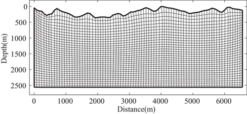
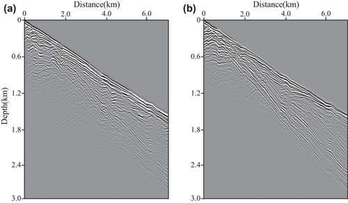
Our second model uses a Canadian Foothills model (Fig. 16). In our modification, the size of the model is 6672 metre x-extent and 2672 metre z-extent with a spatial grid interval of 8 metre × 8 metre in the x- and z-directions. The grid discretization of the Canadian Foothills model with surface topography in the Cartesian coordinates is shown in Fig. 17. Figure 18 shows a one-wavelength smoothed version of the Canadian Foothills model in the curvilinear coordinates as the migration velocity model. The constant density is 2.0 g/cm3. The fixed-spread acquisition geometry is made up of 104 explosive P-wave sources located at 8 metre depth. The source function is a Ricker wavelet with a dominant frequency of 25 Hz. The elastic synthetic data are recorded by 834 two-component receivers located at 8 metre depth. The source interval is 64 minutes, and the receiver interval is 8 minutes. The time step is 0.6 milliseconds and the recording time is 3 seconds. Figure 19 illustrates the synthetic shot records obtained from P- and S-wave separated Born modelling in curvilinear coordinates.


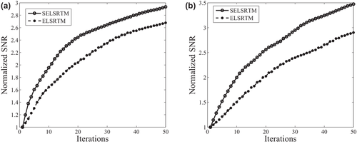
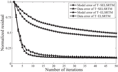
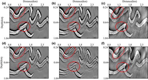
We perform our T-SELSRTM and T-ELSRTM methods with 50 iterations for the two-component synthetic data (the first shot are shown in Fig. 20) generated from the Canadian Foothills model. Figure 21 shows reflectivity of the Canadian Foothills model in the curvilinear coordinates, which can be regarded as true images. Figures 22 and 23 display the migration images obtained from our T-SELSRTM and T-ELSRTM, respectively. Compared with T-ELSRTM images, our T-SELSRTM method generates higher-resolution images of the fault zone and there are some improvements of SNR because when conducting our T-SELSRTM imaging, the P- and S-wave fields are separated to image, thus suppressing the crosstalk artefacts between P- and S-wave. In addition, we also provide the model and the data residual convergence curves for our T-SELSRTM and T-ELSRTM as shown in Fig. 24. The model residual is the L2 misfit between the true reflectivity model and the updated reflectivity model. The data residual curves are calculated by the L2 misfit between the observed data and synthetic data. The convergence curves illustrate the decreases of the model and the data residual over iterations for both our T-SELSRTM and T-ELSRTM. But for the convergence speed of the model and the data residual curves, our T-SELSRTM is faster than T-ELSRTM. Note that the model and data residuals of our T-SELSRTM converge to smaller values than those of T-ELSRTM. Therefore, our T-SELSRTM produces higher-resolution, higher SNR images with faster residual convergence speed than that of conventional T-ELSRTM. Figure 25 shows images after 50 iterations obtained from the conventional ELSRTM. The SNR of this imaging result is low because of the spurious diffractions caused by the surface topography. To better compare the resolution and SNR in the three images, we show the enlarged images of the fault zone in the same coordinates (Fig. 26). The results indicate that the images from our method are the most balanced and continuous as shown by the red ellipse. The computational cost of the proposed T-SELSRTM is more than that of T-ELSRTM and ELSRTM, but the computational time of the proposed method when the misfit decreases to 0.1 is the minimum (shown in Table 1).



DISCUSSION
In this section, we use the Canadian Foothills model to discuss our method's sensitivity to stochastic noise, migration velocity and surface elevation errors. The acquisition geometry and model parameters are the same as Example 2.
Analysis of noise sensitivity
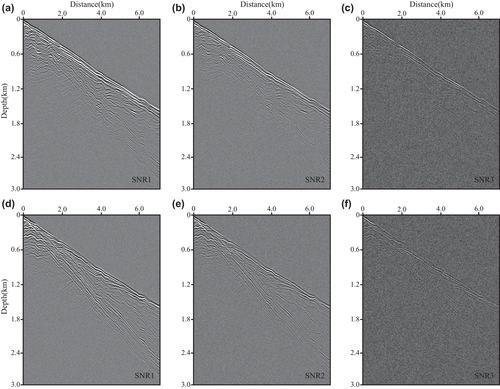
 (39)
(39)
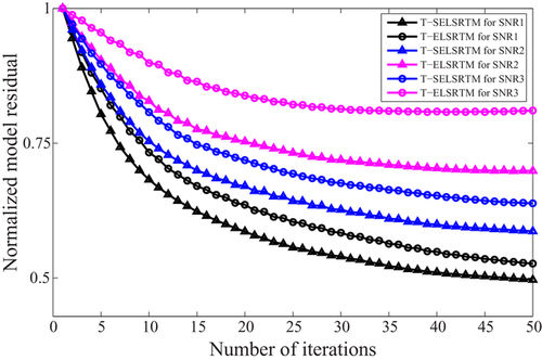
Analysis of starting velocity error sensitivity
 (40)
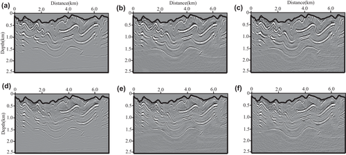
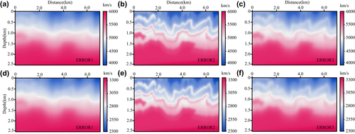
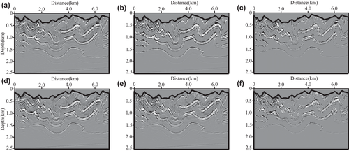
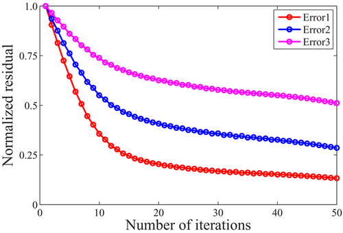
(40)The velocity errors between the migration velocity and the original one are ERROR1 (7.32% smoothed error), ERROR2 (3.84% smoothed error and 2% random error) and ERROR3 (6.44% smoothed error and 4% random error). Figure 30 displays migration velocity models with different errors. Figure 31 shows images of 50 iterations obtained from T-SELSRTM using migration velocity models with different errors. In these results, Fig. 31(a,d) (ERROR1) and Fig. 31(b,e) (ERROR2) show acceptable imaging results. The convergence curves of the data residual over iterations when using imperfect migration velocities are illustrated in Fig. 32. The convergence curves for the three cases converge to different values with different convergence speed, which suggest that our T-SELSRTM method also needs good migration velocities as other LSRTM method.
Analysis of surface elevation error sensitivity
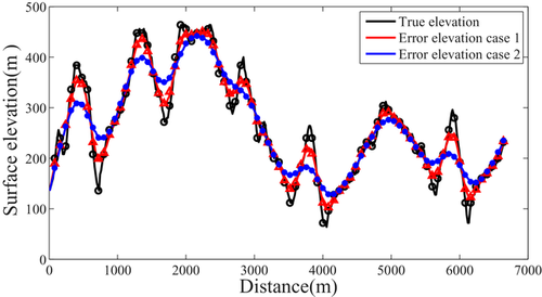
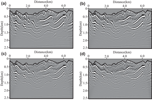
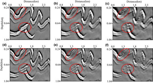
At last, we study the sensitivity of our T-SELSRTM method to the surface elevation. In this section, we use two error surface elevations as shown in Fig. 33. In this figure, the black, red and blue lines denote the true elevation, error elevation case 1 and error elevation case 2. The T-SELSRTM is performed in the curvilinear coordinates, where the Canadian Foothills model with extreme surface topography is conformal to two different moderate surfaces. Figure 34 illustrates images after 50 iterations obtained from T-SELSRTM using different error elevations. For better comparison, we also give the partial zoomed views of images from T-SELSRTM using the true elevation (Fig. 35a,d), error elevation 1 (Fig. 35b,e) and error elevation 2 (Fig. 35c,f). In these results using error elevations, there are some obvious low-frequency noise and false imaging noise. In addition, the amplitude is discontinuous, unclear and unbalanced in some complex structures, especially in high-steep regions. We can conclude that to yield better images, the proposed method needs an accurate surface elevation, which can be obtained by the global positioning system.
CONCLUSIONS
We have presented a topographic separated-wavefield elastic least-squares reverse time migration method that utilizes wavefield-separation demigration equations and gradient formulas in the curvilinear coordinates for the imaging purpose. The main idea is to derive the demigration equations and gradient formulas with respect to vp and vs by applying the wave-separated elastic velocity–stress wave equations in the curvilinear coordinates. Our method is shown to produce higher quality images with less P- and S-wave crosstalk artefacts than conventional elastic least-squares reverse time migration and topographic elastic least-squares reverse time migration. Numerical tests on a three-topographic-layer with anomalies model and the Canadian Foothills model demonstrate that our topographic separated-wavefield elastic least-squares reverse time migration produces higher-resolution, higher SNR images with faster residual convergence speed than that of conventional elastic least-squares reverse time migration and topographic elastic least-squares reverse time migration. The reason is that the proposed topographic separated-wavefield elastic least-squares reverse time migration method can suppress severe spurious diffractions from complex topographic surface conditions by using curvilinear grids and reduce the P- and S-wave crosstalk artefacts by separating the P- and S-wave. We also prove that our topographic separated-wavefield elastic least-squares reverse time migration is less sensitive to noise compared with topographic elastic least-squares reverse time migration and needs good migration velocities and an accurate surface elevation as other least-squares reverse time migration methods.
ACKNOWLEDGEMENTS
This research is supported by the seismic wave propagation and imaging (SWPI) group of China University of Petroleum (East China). This research is supported by the National Natural Science Foundation of China (41774133), the National Science and Technology Major Project of the Ministry of Science and Technology of China (2016ZX05024-003-011), the Open Funds of SINOPEC Key Laboratory of Geophysics (wtyjy-wx2018-01-06) and the Fundamental Research Funds for the Central Universities (19CX02010A).
APPENDIX: VERIFICATION FOR THE SEPARATED FIRST-ORDER P- AND S-WAVE EQUATION IN THE CURVILINEAR COORDINATES
We use two steps to verify the separated P- and S-wave equation (equation (13)):
Step one: Verifying that equation (13) has accurate solutions, which satisfy the velocity–stress wave equation in the curvilinear coordinates (equation 11).
 consists of P-wavefield
  and S-wavefield
  :
:
 (A1)
(A1)The first and second equations of equation 11 (equation (11.1)–(11.2)) can be obtained by adding equation (13b.1)–(13b.2) and equation (13c.1)–(13c.2) together. Therefore, we can draw the conclusion that equation (13) has accurate solutions.
Step two: Verifying that equations 13b and 13c produce curl-free P-wave and divergence-free S-wave, respectively.
 (A2)
(A2)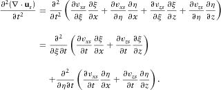 (A3)
(A3)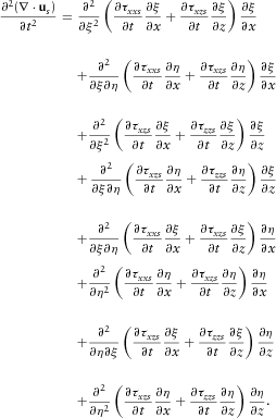 (A4)
(A4)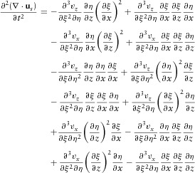 (A5)
(A5) (A6)
(A6) is a non-linear function. Therefore,
 (A7)
(A7) (A9)
(A9) (A10)
(A10)So  . Therefore, equation (13) produces curl-free P-wave and divergence-free S-wave.


 ,
, ,
, and
and  are given by (Fornberg
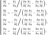
 yields
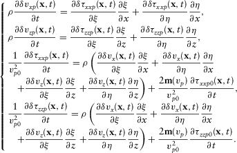
 to equation
