The Relative Volatility of Commodity Prices: A Reappraisal
We thank Olivier Cadot, Jeffrey Frankel, Caroline Freund, Gaston Gelos, Kaddour Hadri, Antoine Heuty, Bernard Hoekman, Mico Loretan, Mustapha Nabli, Chris Papageorgiou, Jim Rowe, and Liugang Sheng for useful comments and discussions. All remaining errors are ours. The views expressed in this paper are those of the authors and do not necessarily reflect those of the International Monetary Fund or of the World Bank, their Board of Directors, or the countries they represent.
Abstract
This article studies the relative volatility of commodity prices by examining a large dataset of monthly prices observed in international trade data taken from the United States between 2002–2011. The evidence presented here suggests that, on average, prices of individual primary commodities are less volatile than individual manufactured goods prices. Furthermore, robustness tests suggest that these results are not likely to be due to alternative product classification choices, differences in product exit rates, measurement errors in the trade data, or the aggregation level of the trade data at the 10-digit level of the Harmonized System of products classification.
Are the international prices of primary commodities more volatile than those of manufactured goods? This question has important implications for macroeconomic and developmental policies such as hedging against volatility and diversifying away from the commodity sector (Arezki, Lederman, and Zhao 2011). The conventional wisdom expressed in academic and policy circles is that commodity prices are more volatile than manufactured goods prices, although the cited evidence usually refers to composite indices of numerous goods and commodities. For instance, graphic evidence provided in The United Nations Conference on Trade and Development (UNCTAD) (2008) suggests that commodity price indices were more volatile than an index of manufactured goods prices from 1970–2008. Some authors, including Jacks, O'Rourke, and Williamson (2011) and Radetski (2008), have argued that commodities' higher price volatility is more often assumed than tested. To remedy this deficiency, the present paper systematically tests whether commodity price volatility is higher than that of manufactured goods prices.
Conceptually, there are good reasons to expect that commodity prices are relatively volatile. One reason is that commodities, by definition, are goods that retain their qualities over time, which allows economic agents to use them as financial assets. This might be the case of gold and other commodities whose prices tend to rise amidst global financial uncertainty. Caballero, Farhi, and Gourinchas (2008), for example, argued that the volatility of commodity prices could be due to the lack of a global safe asset (besides U.S. Treasury Bills). An earlier study argued that commodity price volatility was fueled by stockpiling policies intended to secure access to food or fuel during times of relative scarcity (Deaton and Laroque 1992). These mechanisms add price volatility because of unavoidable asymmetric stockpiling constraints; that is, the stockpile of commodities cannot be negative. Yet another potential explanation is the lumpiness of exploration investments in mining, which results in inelastic supply in the short run (Deaton and Laroque 2003). Finally, more traditional economic analysis of the effects of random demand shocks on homogeneous goods (i.e., commodities) and differentiated goods (i.e., manufactured products) also suggests that the resulting price volatility of the latter would tend to be lower as monopolist suppliers of differentiated products could maximize profits by reducing supply in response to negative demand shocks, thus partially stabilizing the prices of differentiated goods.
However, there are also good reasons to expect a higher level of volatility for differentiated manufactured goods. Product innovation and differentiation itself might contribute to price volatility by producing frequent shifts in residual demand for existing varieties. Indeed, the trade literature (e.g., Schott 2004) has acknowledged the wide dispersion in unit values (a proxy for prices) within narrowly defined product categories in the United States import data at the 10-digit level of the Harmonized System (HS). Also, the demand for differentiated products might be more unstable with respect to household and aggregate income shocks than demand for basic commodities. For instance, the demand for fuel and food might decline proportionately less than the demand for automobiles or electronics when incomes fall.
In spite of these contradictory predictions, there are few analyses that systematically compare the volatility of commodity and manufactured goods prices. An important exception is the historical study by Jacks, O'Rourke, and Williamson (2011), who examined the volatility of domestic prices since 1700 in several countries. These authors provide evidence that commodities have always shown greater price volatility than manufactured goods by using monthly price quotes for various items including food, agriculture, minerals, and final goods. However, their study covered only a few commodities due to data constraints. Another important exception is the study by Mintz (1967), who documented that U.S. export prices for manufactured products were less volatile than raw materials from 1880–1913 and 1921–1961, although Mintz also used price indices covering multiple goods in each price index. More recent analyses of the evolution and volatility of the average price of baskets of commodities relative to the average price of a basket of manufactured goods–usually the manufacturing unit value index (MUV) constructed by the International Monetary Fund–are omnipresent in the literature and policy documents (e.g., Cashin and McDermott 2002; UNCTAD 2008; Calvo-Gonzalez, Shankar, and Trezzi 2010).
Figures 1 and 2 show the time series of aggregate price indices for various definitions of primary commodities. In particular, figure 1 shows U.S. import and export (aggregate) price indices for manufactured goods, as well as the widely-used IMF commodity price indices and sub-indices, namely non-fuel primary commodities and energy products (IMF Primary Commodity Price Tables are available at: http://www.imf.org/external/np/res/commod/index.aspx). Figure 2 shows UNCTAD's commodity price index, another of the widely-used commodity price indices. These series seem to corroborate conventional wisdom, as commodity prices appear to be more volatile than non-commodity prices. The present article challenges this conventional wisdom by providing a new stylized fact on the relative volatility of primary commodity prices using data from U.S. imports data at the 10-digit level of aggregation in the HS nomenclature.
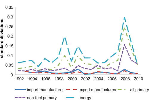
Volatility of aggregate price indices: IMF commodity indices Notes: The figure shows the evolution of the annualized standard deviations of Hodrick-Prescott filtered price series. The aggregate price indices for all primary, non-fuel primary, and energy goods are from IMF Primary Commodity Price Tables (2005=100). The aggregate price indices for import and export manufactured goods are from the Bureau of Labor Statistics (2000=100). The latter data were available using the Standard International Trade Classification from 1993 to 2005 and available using the North American Industry Classification System from 2005 to 2010. We constructed the series for 1993–2010 by setting the same index value for December 2005.
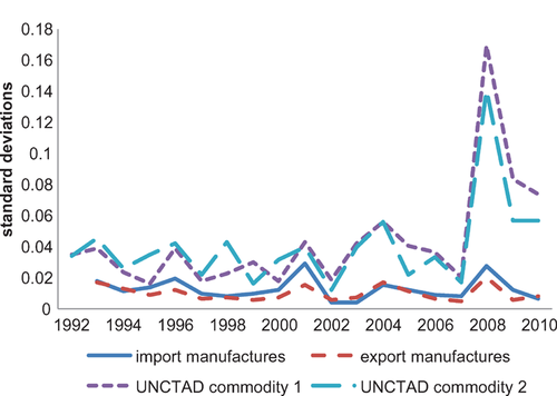
Volatility of aggregate price indices: UNCTAD commodity indices Note: The figure shows the evolution of the annualized standard deviations of Hodrick-Prescott filtered price series. Commodity price indices are from UNCTAD Stat (2000=100). The UNCTAD commodity 1 price index is originally in current dollars, whereas the UNCTAD Commodity 2 is in Special Drawing Rights. The aggregate price indices for import and export manufactured goods are from the Bureau of Labor Statistics (2000=100). The latter data were available using the Standard International Trade Classification from 1993 to 2005 and available using the North American Industry Classification System from 2005 to 2010. We constructed the series for 1993–2010 by setting the same index value for December 2005.
This article contributes to several strands of the literature. First, it contributes most directly to the literature on commodity prices behavior. This literature does not necessarily compare commodity prices to non-commodity prices, but focuses on the former. For instance, Deaton and Laroque (1992) used coefficients of variation for aggregated price indices as a measure of volatility to analyze the volatility of 13 commodities; they argue that “commodity prices are extremely volatile,” but do not provide an explicit comparison with non-commodity price volatility.1 To the best of our knowledge, this article is the first to compare the volatility of individual primary commodity prices with the volatility of manufactured goods prices based not on aggregate indices, but on disaggregated monthly data.
This article also contributes to the literature comparing the evolution of commodity prices relative to manufactured products. For instance, Harvey et al. (2010) employ a unique data set and new time-series techniques to reexamine the existence of trends in the relative prices of primary commodities. The data set comprises 25 commodities and provides a new historical perspective spanning from the seventeenth to the twenty-first century. Results show that many primary commodity prices have followed a downward trend for a prolonged period. Instead of focusing on trends, our paper focuses on the differences in the second moments of commodity price series, namely the volatility of commodity prices relative to the volatility of manufactured goods prices.
Further, this article contributes to the literature on the “resource curse” that has focused on the adverse effect of resource endowments on economic growth (e.g., Lederman and Maloney 2007; Van der Ploeg 2011; Frankel 2012). This literature has documented several channels through which the curse may operate, including the transmission of commodity export prices to the domestic economy. If commodity prices are intrinsically more volatile than the prices of manufactured goods, natural resource endowments could result in macroeconomic volatility. This literature has assumed rather than tested the premise that primary commodity prices are inherently more volatile than those of individual manufactured goods. Our contribution is to unveil empirical regularities on the relative volatility of commodity prices so as to provide a sound basis for the policy debate.
The rest of the article is organized as follows. The second section presents monthly data from the U.S. international trade records from 2002–2011 covering more than 18,000 goods. The third section presents the main results. The fourth section provides an array of robustness tests, and the fifth section concludes.
Data
Our data come from trade records of the United States, classified at the 10-digit level of the HS trade classification. We use monthly import data from January 2002 to April 2011. The data were obtained from the Foreign Trade Division of the U.S. Census Bureau (data available at: https://usatrade.census.gov/). From these data, prices were computed as the ratio of import values to quantities; these unit values are used as our proxy for product prices.
In total, the dataset covers 26,459 product categories. However, not all product categories have information on prices; 7,976 products do not. Also, the analysis of volatility requires data for extended periods of time, and we dropped products that do not have price data for at least 36 consecutive months. The final data set thus covers 12,955 products.2
Our benchmark analysis focuses on U.S. imports data rather than on exports data for two reasons. First, imports data are generally less afflicted by measurement errors than exports data, because imports are subject to tariffs and are more likely to be inspected than exports. Second, U.S. imported products are more numerous and diverse than exports. In fact, the U.S. reports twice as many imported as exported goods. Also, 17% of imports are commodities compared to only 4% of exports. While studying the pattern of U.S. exports may be relevant for a specific analysis of the United States, it is essential for our general analysis to use imports data.3
It is noteworthy that this sample covers years of historically high volatility in real commodity prices, levels that were perhaps surpassed only in the early 1970s (see, e.g., Calvo-Gonzalez, Shankar, and Trezzi 2010). Consequently, if there is a period selection bias in the data, it would probably bias commodity price volatility upwards. But, again, such historical analyses focus on commodity prices relative to an aggregate price index of non-commodity goods, which might be misleading.
As a starting point, the analysis focuses on aggregate price indices—see figures 1 and 2. A relevant issue in this type of analysis concerns the definition of commodities. The International Monetary Fund (IMF) has one such classification that includes non-fuel, energy and all primary commodities. The United Nations Conference on Trade and Development (UNCTAD) also has a definition that includes some commodities that are not in the IMF's data set, such as cottonseed oil and manganese ore. Appendix 1 lists the commodities included under both definitions. In addition, it is easy to tell which goods are manufactured in the North American Industry Classification System (NAICS). At the two-digit level, chapters 31–39 of the NAICS are classified as manufactured goods.
Since the data on import prices from the United States are classified according to the HS, we used concordance tables between the HS and the NAICS.4 To identify commodities among the non-manufactured goods (that is, the products in the NAICS that are not listed in chapters 31–39), we match the HS data to the IMF and UNCTAD commodity classifications. To match the HS product categories to the IMF and UNCTAD lists of commodities, we used the names of the commodities as keywords to find matching product descriptions in the HS trade data. In sum, we use the NAICS classification and the concordance table between NAICS and the HS to identify manufactured goods in our trade data, and then use the names of commodities identified by the IMF and UNCTAD to identify the commodities in the remaining non-manufactured products in the HS classification.
To assess the volatility of individual goods prices it is important to de-trend the price series. There are two main reasons for this; the first is purely statistical. Since many of the series contain a unit root, their standard deviations change over time and diverge to infinity. Consequently, it would be inappropriate to compute using standard deviations of such a non-stationary series as a measure of volatility. The second reason relates to the short-run nature of volatility. Since we are only interested in volatility and not in secular changes, we only exploit the cyclical component of the various series to compute the standard deviation. We report our results based on the Hodrick-Prescott filtered series, but all results reported herein hold with alternative filters, including the Christiano-Fitzgerald filter, the Baxter-King band-pass filter, and first differences.5 There is thus no concern that the main result presented in this article is driven by the choice of filtering method. In all three cases, we measure volatility with the standard deviation of de-trended price series. Logarithms are taken for all price series prior to de-trending so that the standard deviations are scale invariant. After calculating the standard deviations for each 10-digit product, we compare the distribution of volatilities across groups of goods, namely commodities versus manufactured goods.
Results
As mentioned above, we are interested in comparing the distribution of price volatilities across broad categories of goods.
Product “Re-Classification”
In the HS classification, the goods classified as machinery and electrical equipment have the highest average volatility—see table 1. Table 2 provides summary statistics for the goods classified as primary commodities and manufactured goods for a period spanning January 2002 to April 2011, based on the NAICS-IMF classification, after finding the best concordance between the two classifications. Over 92% of the products are classified as manufactured goods and have, on average, higher volatilities than the primary commodities. Furthermore, the cumulative distribution functions (CDFs) in figure 3 show that the price volatility of manufactured goods dominates both that of primary commodities and that of other (unmatched) goods.
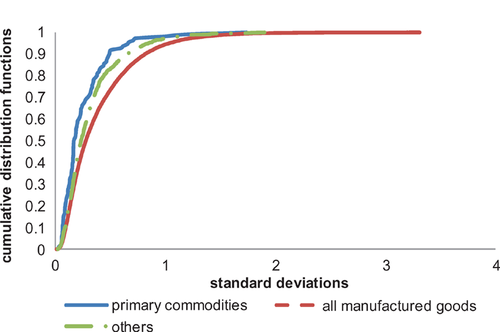
Cumulative distribution functions of price volatilities for products with uninterrupted price series Note: The figure shows the cumulative distribution functions (CDFs) of the standard deviations of Hodrick-Prescott filtered series of individual goods prices (in natural logarithms). The included products are those with prices available for at least 36 consecutive months. Data are from the Foreign Trade Division of the U.S. Census Bureau.
For the sake of completeness, figure 4 plots the volatility CDF of primary commodities based on the IMF commodity price table data, the previously defined group of manufactured products and primary commodities, and a more narrow set of manufactured goods classified as “computers.” The latter appear to have the highest volatility distribution, followed by the large group of all manufactured goods.
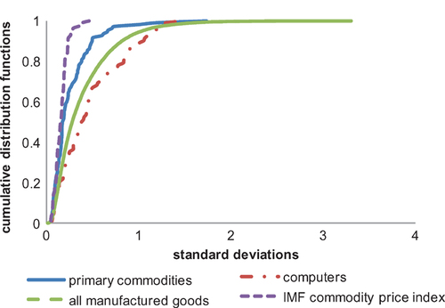
Cumulative distribution functions of price volatilities for various product categories Note: The figure shows the cumulative distribution functions (CDFs) of the standard deviations of Hodrick-Prescott filtered series of individual goods prices (in natural logarithms). The volatility CDF of IMF commodities is based on the IMF commodity price data, manufactured products and primary commodities are based on the U.S. import data from the Foreign Trade Division of the U.S. Census Bureau (see text for details), and a more narrow set of manufactured goods are classified as “computers.”
| HS | Description | Number of Goods | Mean | Minimum | Maximum |
|---|---|---|---|---|---|
| 01–05 | Animal & Animal Products | 505 | 0.223 | 0.023 | 1.499 |
| 06–15 | Vegetable Products | 592 | 0.271 | 0.027 | 1.736 |
| 16–24 | Foodstuffs | 662 | 0.219 | 0.013 | 1.131 |
| 25–27 | Mineral Products | 201 | 0.376 | 0.033 | 1.435 |
| 28–38 | Chemicals & Allied Industries | 1,564 | 0.425 | 0.038 | 2.543 |
| 39–40 | Plastics/Rubbers | 420 | 0.280 | 0.026 | 1.551 |
| 41–43 | Raw Hides, Skins, Leather & Furs | 220 | 0.444 | 0.071 | 1.528 |
| 44–49 | Wood & Wood Products | 808 | 0.293 | 0.028 | 2.206 |
| 50–63 | Textiles | 2,630 | 0.410 | 0.028 | 1.583 |
| 64–67 | Footwear/Headgear | 341 | 0.301 | 0.016 | 1.163 |
| 68–71 | Stone/Glass | 385 | 0.415 | 0.019 | 2.750 |
| 72–83 | Metals | 1,448 | 0.271 | 0.044 | 1.678 |
| 84–85 | Machinery/Electrical | 2,021 | 0.526 | 0.034 | 3.310 |
| 86–89 | Transportation | 384 | 0.382 | 0.028 | 2.370 |
| 90–97 | Miscellaneous | 773 | 0.502 | 0.033 | 2.326 |
| 98–99 | Service | 1 | 0.406 | 0.406 | 0.406 |
| Total | 12,955 | 0.382 | 0.013 | 3.310 |
- a Source: Authors' calculations, based on data from the Foreign Trade Division of the U.S. Census Bureau.Note: The table shows the mean, minimum and maximum of the standard deviations of Hodrick-Prescott filtered series of product-group prices (in natural logarithms).
| Description | Number of Goods | Mean (standard deviation) | Minimum (standard deviation) | Maximum (standard deviation) |
|---|---|---|---|---|
| Primary commodities | 110 | 0.257 | 0.031 | 1.736 |
| Manufactured goods | 12,006 | 0.387 | 0.013 | 3.310 |
| Others | 839 | 0.316 | 0.023 | 1.897 |
| Total | 12,955 | 0.382 | 0.013 | 3.310 |
- a Source: Authors' calculations, based on data from the Foreign Trade Division of the U.S. Census Bureau.
Thus, the data on price volatility at the level of individual products suggest that manufactured goods prices are more volatile than commodities prices. This result is at odds with figure 1. We argue that the use of aggregate indices in comparing prices across classes of goods is subject to an aggregation bias. That is, some price swings in one direction cancel out swings in the other direction, which makes for an overall index that looks more stable than its components.6 Of course this effect is also at play in commodity price indices, but there are far fewer commodities than manufactures, so fewer prices cancel each other out. According to the NAICS, manufactures account for more than 90% of the goods in our data set. Nonetheless, since the analysis compares the whole distribution of volatilities within categories of goods, we next need to establish that the observed differences in the CDFs are statistically significant.
Formal Tests of Stochastic Dominance
Delgado, Farinas, and Ruano (2002) provide a non-parametric test for assessing the difference between cumulative distribution functions; it is a two-step test for first-order stochastic dominance. The first step is a one-sided test of the null hypothesis that the difference between the two cumulative distribution functions is equal to or less than zero. The second step is a two-sided test of the null hypothesis that the two CDFs are equal. If the one-sided test is not rejected, then this is interpreted as evidence of weakly stochastic dominance. A rejection of the equality of the two CDFs in the two-sided test indicates strict stochastic dominance.
 (1)
(1) denotes the empirical cumulative distribution function. The test statistic for the two-sided test examines the distribution of the absolute value of the differences (as opposed to the differences) between the two empirical distributions:
 (2)
(2)Robustness
This section tests the robustness of our surprising finding that prices of commodities are less volatile than those of manufactured goods. This finding could be misleading for at least five reasons. First, some products tend to disappear from the sample. If most product exits are observed within the group of manufactured goods, then it is possible that the observed volatility of manufactures might be biased upward, driven by product destruction rather than by within-product price fluctuations. Second, the trade data on unit values comes from ratios of reported values over reported quantities. Hence, it is worth examining the volatility of quantities. Third, the key distinguishing feature of commodities is their relative lack of product differentiation over time, and this characteristic might not be neatly identified in the ad hoc categorizations used by the IMF, UNCTAD, or in the NAICS. Fourth, measurement errors in unit values may be an important explanation for our main results. Fifth, even at the ten-digit level of aggregation in the HS nomenclature, each product code might include multiple varieties of products. Thus, the level of aggregation might affect the estimates of price volatilities. We address these concerns below.8
Product Destruction
An easy way to examine the influence of product destruction on the previous results is to limit the analysis to a constant sample of products. For this constant sample, we chose goods that have price information from January 2002 to April 2011. Thus, our sample is reduced to 7,842 goods, which is about 60% of the total number of goods (12,955) in the benchmark sample. Indeed, table 3 shows that there is quite a bit of product exit in manufactured products. There is also a notable increase in the number of entering and exiting products in 2007, which is very likely due to changes in the trade classification and reporting systems. The supplementary appendix online reports formal stochastic dominance test results that provide evidence that our main findings are robust across the two sub-samples from 2002–2006 and 2007–2011. Further, figure 5 shows that even when considering a constant sample of products, our main result remains intact: commodities prices appear to be less volatile than manufactured goods prices.
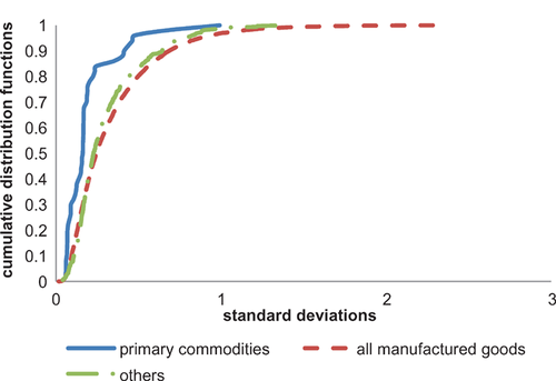
Cumulative distribution function of price volatility for goods available for the whole period Notes: The figure shows the cumulative distribution functions of the standard deviations of Hodrick-Prescott filtered series of individual goods prices (in natural logarithms). The goods represented are those with price (unit value) data available for the whole sample period (Jan. 2002–Apr. 2011). Data are from the Foreign Trade Division of the U.S. Census Bureau.
| Number of Exiting Goods | Number of New Goods | |||||||
|---|---|---|---|---|---|---|---|---|
| Year | Commodities | Manufactured Goods | Others | Total | Commodities | Manufactured Goods | Others | Total |
| 2003 | 1 | 90 | 8 | 99 | 0 | 115 | 10 | 125 |
| 2004 | 1 | 81 | 5 | 87 | 0 | 97 | 0 | 97 |
| 2005 | 3 | 70 | 9 | 82 | 0 | 94 | 7 | 101 |
| 2006 | 0 | 57 | 6 | 63 | 0 | 113 | 2 | 115 |
| 2007 | 19 | 1,510 | 225 | 1,754 | 20 | 1,320 | 216 | 1,556 |
| 2008 | 0 | 37 | 5 | 42 | 1 | 73 | 6 | 80 |
| 2009 | 1 | 40 | 11 | 52 | 2 | 63 | 12 | 77 |
| 2010 | 3 | 55 | 5 | 63 | 3 | 33 | 2 | 38 |
| 2011 | 3 | 307 | 67 | 377 | 10 | 108 | 16 | 134 |
- a Source: Authors' calculations, based on data from the Foreign Trade Division of the U.S. Census Bureau.
Volatility of Quantities
Thus far, we have used unit values to compute measures of price volatility. It is important to keep in mind that quantities may adjust to prices, and it is worth exploring whether the difference in volatilities between primary commodity and non-primary goods prices is evident in quantities. We thus re-computed the volatility for quantities, both for individual commodities and for manufactures. Figure 6 shows that our main result—that individual commodity prices are less volatile than those for manufactures—holds for import quantities as well.
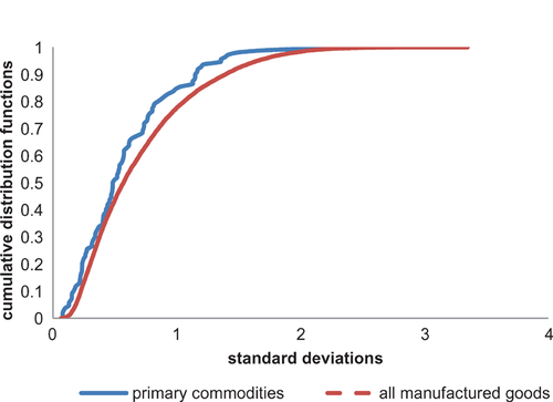
Cumulative distribution functions of the volatilities of import quantities Notes: The figure shows the cumulative distribution functions of the standard deviations of Hodrick-Prescott filtered series of individual product quantities (in natural logarithms). Data are from the Foreign Trade Division of the U.S. Census Bureau.
Homogeneous versus Differentiated Products
Rauch (1999) provided an intuitive classification of homogeneous and differentiated goods. Homogeneous goods are traded globally in organized exchanges, whereas differentiated goods are not. An intermediate category was presented in Rauch (1999), and is composed of goods for which no formal exchanges (organized markets) exist, but for which there are “reference prices.” Rauch provided a concordance between the Standard International Trade Classification (SITC) and his three categories. We used the SITC-HS concordance table to then classify our sample of products into Rauch's three groups. In our sample, 95% of the manufactured goods appear in the bin of differentiated goods, whereas only 35% of the commodities were classified as differentiated products. Thus, there was a notable overlap, albeit not enough to overturn the main findings: figure 7 indicates that the most volatile products are differentiated manufactured goods.
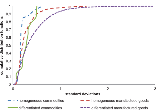
Cumulative distribution functions of price volatilities of differentiated and homogenous goods Notes: The figure shows the cumulative distribution functions of the standard deviations of Hodrick-Prescott filtered series of individual goods prices (in natural logarithms). Data are from the Foreign Trade Division of the U.S. Census Bureau.
Measurement Errors
One possible caveat to our results is that measurement errors in the unit values may be an important driver of the difference in the observed—as opposed to the true—price volatility between commodity and manufactured goods.9 One potential source of measurement error is that goods with low import values may be disproportionately more subject to measurement error. Following Hummels and Klenow (2005) and Feenstra, Romalis and Schott (2002), we re-computed the price volatility CDFs for various groups of products after dropping goods with a monthly import value below a given cut-off. Specifically, we dropped goods below US$50,000 in import value, which resulted in a drop of 6% (805 goods) of the total number of products. Interestingly, the dropped goods were evenly distributed across commodity and manufactured goods. Our main results regarding the higher volatility of manufactured goods unit values were confirmed after dropping goods with low import values.
Another potential source of concern is that using the standard deviation as a measure of dispersion may assign disproportionate importance to outliers, which in turn may lead to overestimation or underestimation of the relative volatility of commodity prices. Indeed, a standard deviation, being the square root of the mean squared deviation of the price from the time-average of the price series, implicitly assigns more weight to outliers. To address this issue we used an alternative set of indicators of dispersion, namely an inter-deciles range given by the difference between the first and the ninth deciles, and the inter-quartile range given by the difference between the upper and lower quartiles. Once again, when re-computing the price volatility CDFs, our main results regarding the higher volatility of manufactured goods unit values were confirmed using these alternative measures of dispersion. While it is impossible to argue with absolute certainty that measurement error does not drive our main results, this evidence suggests that measurement errors that disproportionately affect unit values of manufactured goods are unlikely to be the main source of the difference in volatilities with respect to commodities.
Level of Aggregation and Product Varieties in the Trade Nomenclature
Lastly, we explore the role of aggregation level in the trade classification system to ascertain whether our results might be due to the existence of multiple product varieties and even various types of products, especially among manufactured products, within the narrowly-defined product categories at the 10-digit level of the HS. It is plausible that the CDFs of product-price volatilities might reflect price fluctuations of many products. The results might thus be biased in either direction. If the product categories include many product varieties and their underlying unit values do not co-move, then the observed volatilities of the manufactured products might be under-estimated. If the underlying prices do co-move, then the price volatilities might be either over-stated or unbiased, depending on the nature of the co-movement of the underlying prices. To assess whether variety bundling within product categories biases the estimated volatilities, we examined the relationship between the level of aggregation of the trade nomenclature and the differences in the CDF of volatilities between commodities and manufactured products. The idea is to assess whether the level of aggregation affects the estimated differences in the CDFs of price volatilities between commodities and manufactured goods. If those differences are smaller at higher (than 10 digits) levels of aggregation, then we can expect the differences to be larger if we were to find even more disaggregated price data at the product level. This seems to be a practical way to proceed, because we do not have access to data at higher levels of disaggregation than the data at 10 digits.
The results for the stochastic dominance tests with the data at different levels of aggregation are shown in table 4. At all levels of aggregation, we fail to reject the null hypothesis that manufactured goods prices are more volatile than those of commodities (again, using the NAICS-IMF classification of products as manufactured or commodities). In contrast, we can reject the null that commodities prices are more volatile than manufactured goods prices at the 10- and 8-digit levels of aggregation, but the significance disappears at higher aggregation levels. Likewise, we can reject the null of the two-sided test that the two CDFs are equal only at the 10- and 8-digit level of aggregation. That is, it seems that the differences in the CDFs of price volatilities become more pronounced with the number of digits in the product code of the HS nomenclature. Thus, we conclude that our estimates of the differences using the 10-digit level data are a floor rather than a ceiling, and commodity prices would likely become relatively more stable than those of manufactured goods if we were able to use a more precise product classification system.
| Level of Aggregation in the HS Nomenclature | ||||||
|---|---|---|---|---|---|---|
| Stochastic Dominance Test: Null Hypothesis | 10 | 8 | 6 | 4 | 2 | |
| Manufactured Price Volatility Weakly Dominates Commodity Price Volatility | Kolmogorov-Smirnov test statistic | 0.034 | 0.255 | 0.227 | 0.697 | 0.563 |
| p-value | 0.998 | 0.878 | 0.902 | 0.379 | 0.531 | |
| Commodity Price Volatility Weakly Dominates Manufactured Price Volatility | Kolmogorov-Smirnov test statistic | 2.404 | 1.312 | 0.656 | 0.826 | 0.366 |
| p-value | 0.000 | 0.032 | 0.423 | 0.256 | 0.765 | |
| CDFs of Price Volatilities are Equal | Two-Sided Test p-value | 0.000 | 0.042 | 0.699 | 0.376 | 0.670 |
| No. of manufactured products | 12,006 | 5,788 | 3,598 | 983 | 77 | |
| No. of commodities | 110 | 33 | 26 | 10 | 5 | |
- a Source: Authors' calculations, based on data from the Foreign Trade Division of the U.S. Census Bureau; see text for details.
Conclusions
Conventional wisdom holds that commodity prices are more volatile than the prices of differentiated manufactured products. However, there are economic arguments that both support and counter this perception. The literature has focused on trends and volatilities of price indices ratios composed of multiple commodities and manufactured products. This approach can be misleading, as the use of aggregate indices in comparing prices across classes of goods is subject to aggregation bias.
Our empirical results challenge the conventional wisdom. In fact, the evidence presented in this article suggests that, on average, the prices of individual primary commodities might be less volatile than individual manufactured goods prices. Furthermore, robustness tests suggest that these results are not likely to be due to alternative product classification choices, differences in product exit rates, measurement errors in the trade data, or the level of aggregation of the trade data. Indeed, our estimates with the U.S. trade data at the 10-digit level of aggregation in the HS nomenclature are likely to be a floor estimate of the difference between the volatilities of commodities and manufactured (or differentiated) goods. Hence, the explanation must be found in the realm of economics, rather than measurement.
Caution is required when discussing the policy implications of our main results. Indeed, nearly all developing countries have much smaller economies than major industrialized countries, and are more likely to specialize in exporting commodities. This concentration in their export baskets is associated with volatile terms of trade, so managing external volatility and economic diversification remain important long-term policy challenges for developing countries.
More research is needed to explore the theoretical explanations of these new findings. As mentioned in the introduction, one likely candidate is that product differentiation itself might contribute to price volatility by producing frequent shifts in residual demand for existing varieties. The wide dispersion in unit values within narrowly-defined product categories in the U.S. import data at the 10-digit level of the HS (Schott 2004) supports this view.
Our empirical results also have potentially important implications for the macroeconomics literature. Koren and Teneyro (2007) document that the volatility of country-specific macroeconomic shocks falls with increased levels of development, and that the degree of sectoral concentration declines with development during its initial stages and then increases at later stages. Since sectoral concentration follows an inverted U shape, it is important to focus on empirical regularities not only between sectors, but also within sectors. The evidence presented in this article suggests that using disaggregated data can help shed light on empirical regularities of the nature of shocks within sectors. More research, however, is needed to analyze the covariance of shocks within sectors. From a policy standpoint, knowledge about the nature of shocks and their covariance within sectors could help in the design of policies aimed at hedging against volatility at the firm and sectoral levels.
A Appendix 1. Lists of Commodities under the IMF Primary Commodity Price Tables and UNCTAD Classifications
IMF Primary Commodity Price Tables: Aluminum, bananas, barley, beef, butter, coal, cocoa beans, coconut oil, coffee, copper, copra, cotton, diammonium phosphate (DAP), fish, fish meal, gasoline, gold, groundnuts, groundnut oil, hides, iron ore, jute, lamb, lead, linseed oil, maize, natural gas, newsprint, nickel, olive oil, oranges, palm kernel oil, palm oil, pepper, petroleum, phosphate rock, potash, poultry, plywood, pulp, rice, rubber, shrimp, silver, sisal, sorghum, soybeans, soybean meal, soybean oil, sugar, sunflower oil, superphosphate, swine meat, tea, timber, hardwood logs, hardwood sawnwood, softwood logs, softwood sawnwood, tin, tobacco, uranium, urea, wheat, wool, and zinc.
UNCTAD: Aluminum, bananas, beef, cattle hides, coarse wool, cocoa beans, coconut oil, coffee, copper, copra, cotton, cottonseed oil, crude petroleum, fine wool, fish meal, gold, groundnut oil, iron ore, jute, lead, linseed oil, maize, manganese ore, nickel, non-coniferous woods, palm kernel oil, palm oil, pepper, phosphate rock, plywood, rice, rubber, silver, sisal, soybean oil, soybeans, soybean meal, sugar, sunflower oil, tea, tin, tobacco, tropical logs, tropical sawnwood, tungsten ore, wheat, and zinc.


