Crop Productivity and the Global Livestock Sector: Implications for Land Use Change and Greenhouse Gas Emissions
Petr Havlík ([email protected]) is researcher at the International Institute for Applied Systems Analysis and at the International Livestock Research Institute, Nairobi, Kenya. Hugo Valin ([email protected]), Aline Mosnier ([email protected]) and Michael Obersteiner ([email protected]) are researchers with the International Institute for Applied Systems Analysis, Laxenburg, Austria. Justin S. Baker ([email protected]) is researcher at RTI International. Mario Herrero ([email protected]) and Mariana C. Rufino ([email protected]) are researchers with the International Livestock Research Institute. Erwin Schmid ([email protected]) is Professor at the University of Natural Resources and Life Sciences, Vienna. The research was supported by the EU-funded FP7 project ANIMALCHANGE (grant no. 266018).
This article was presented in an invited paper session at the 2012 AAEA Annual meeting in Seattle, WA. The articles in these sessions are not subjected to the journal's standard refereeing process.
The livestock sector accounts for 30% of global land area and is a major driver of land use change (Geist and Lambin 2002). Steinfeld et al. (2006) calculated that deforestation due to the expansion of pasture and feed crops was responsible for 8% of total anthropogenic CO2 emissions. In addition, methane emissions from enteric fermentation and manure management accounted for 32% and 7%, respectively, of agricultural sector non-CO2 emissions (USEPA 2006). Future developments in the livestock sector will thus have large impacts on global greenhouse gas (GHG) emission levels. The objectives of this paper are: 1) to investigate the particular role played by crop yield increases in the dynamics of livestock production systems; 2) to explore whether these dynamics could lead to sparing of not only cropland but also grassland; and 3) to quantify the implications for related GHG emissions.
Crop yield increases since 1961 have spared 85% of cropland expansion and avoided emissions of some 590 gigatons (Gt) CO2-eq in the crop sector, compared to an alternative scenario without productivity increases (Burney, Davis, and Lobell 2010). In a prospective analysis, Tilman et al. (2011) demonstrated that if the current trends of low intensification in developing regions were to continue, five times more additional cropland (1 billion ha) would be needed and three times more GHG emissions would be emitted by 2050 than under a scenario with agricultural technology improvements. However, neither of these studies considered the indirect effects of increases in crop productivity on the dynamics of the livestock sector, or the extent of grasslands required for livestock production.
Evenson and Rosegrant (2003) showed that without the improvements that took place in crop genetics between 1965 and 2000, food crop prices would have been 35–66% higher. The price reductions generated by crop yield increases should, ceteris paribus, encourage farmers to replace some of the grass in ruminant rations with crops. This would lead to land sparing and related CO2 emission reductions in regions where the feed productivity per unit of area is higher for cropland than for grassland. However, because of the multiple and complex relationships between crop, livestock and land use, clear-cut conclusions about the direction and magnitude of change in land use and GHG emissions cannot be obtained without integrated economic modeling.
In this study we implement the global partial equilibrium model GLOBIOM, which has been used extensively in the past: 1) to analyze the effects of biofuel policies on total GHG emissions balance (Havlík et al. 2011; Frank et al. forthcoming; and Mosnier et al. 2012); 2) to assess the mitigation potential of reduced emissions from deforestation (Böttcher et al. 2012); and 3) to investigate future global challenges in the sector in general (Schneider et al. 2011). The model specifically allows feed requirements to be defined in physical units for each production system. Hence, the substitution of feed crops for grass can be explicitly modeled as a switch from one system to another. To assess the effects of crop yield growth, we first simulate future scenarios with varying crop yield assumptions, and we compare their effects on the structure of production systems, cropland and grassland expansion, and GHG emissions. In a second step, we compare the resulting emission reductions with the efforts that would be needed under mitigation policies without crop yield growth, and discuss their implications for policy-making.
Model
The Global Biosphere Management Model (GLOBIOM) is a partial equilibrium model that covers the agricultural and forestry sectors, including the bioenergy sector. It is used for analyzing medium- to long-term land use change scenarios. In GLOBIOM, the world is divided into 30 economic regions, in which a representative consumer is modeled through a set of isoelastic demand functions. The spatial resolution of the supply side relies on the concept of Simulation Units, which are aggregates of 5 to 30 arcminute pixels belonging to the same altitude, slope, and soil class, and also the same country. For crops, grass, and forest products, Leontief production functions covering alternative production systems are calibrated based on biophysical models like EPIC (Williams 1995). For the present study, the supply side spatial resolution was aggregated to 120 arcminute (about 200 x 200 km at the equator).
Economic optimization is based on the spatial equilibrium modeling approach (Takayama and Judge 1971). The price-quantity equilibrium is computed as in McCarl and Spreen (1980) at the regional level. The model is calibrated to year 2000 FAOSTAT activity levels, and is then recursively solved in 10-year time steps.
Livestock Sector
GLOBIOM incorporates a particularly detailed representation of the global livestock sector. With respect to animal species, a distinction is made between dairy and other bovines, dairy and other sheep and goats, laying hens and broilers, and pigs. Livestock production activities are defined in several alternative production systems adapted from Seré and Steinfeld (1996): for ruminants, grass-based (arid, humid, temperate/highlands), mixed crop-livestock (arid, humid, temperate/highlands), and other, are distinguished monogastrics are split in smallholder and industrial systems. For each species, production system, and region, a set of input-output parameters is calculated based on the approach presented in Herrero et al. (2008). Feed rations are defined as consisting of grass, stovers, feed crop aggregates, and other feedstuffs. Outputs include four meat types, milk, and eggs, and environmental factors (manure production, N-excretion, and GHG emissions). The initial distribution of the production systems is based on Robinson et al. (2011). Switches between production systems allow for feedstuff substitution and for the intensification or extensification of livestock production.
Land Use Change
Six land cover types are distinguished in GLOBIOM: cropland, grassland, short rotation tree plantations, managed forest, unmanaged forest and other natural vegetation. Depending on the relative profitability of the individual activities, and on the inertia constraints, the model can switch from one land cover type to another. Comprehensive greenhouse gas accounting for agriculture and land use change is implemented in the model. A detailed description of these accounts and other additional background information are provided in Havlík et al. (2011) and Mosnier et al. (2012).
Scenarios
The extent to which future crop yields will follow past trends is highly uncertain and depends on the capacity of farmers to invest in better technologies and varieties, and to improve their management to achieve best practices in their natural and institutional environment. We now look at the effect of four contrasting scenarios of crop yield evolution through 2030.
The baseline scenario (B) shows the yield growth trends observed over the last 30 years. The average growth rates for each crop in each region are computed by an ordinary least square regression on FAO time series for the period 1980–2010. Yields are then extrapolated assuming a linear trend, which best fits past data (Fischer, Byerlee, and Edmeades 2009). This corresponds to an average annual growth rate of 1% for developed countries, and 1.3% for developing countries for 2000–2030. Scenario (S0) is a counter-factual scenario which maintains yields at their 2000 level.
Two other scenarios complement the picture. Convergence scenario (C) assumes that developing regions experience fast technology transfer from developed regions, and significant improvement in their own cultivation techniques.1 For this scenario, the linear slope of developing countries in scenario (B) is doubled, whereas the yield evolution for developed regions remains unchanged. This leads to emerging countries growing at an average annual rate of 2%, and the least advanced countries growing at 2.3% per year. These trends seem achievable in light of the literature that emphasizes the magnitude of yield gaps in developing countries (Lobell, Cassman, and Field 2009). Finally, scenario (S) considers that yield growth rates are only one-half of those in scenario (B).
To isolate the impacts of feed substitution on land use and GHG emissions, we maintain final demand for agricultural products at the level calculated endogenously in the baseline scenario (B). For that scenario, the income effect on future demand follows the FAO assumptions (Alexandratos et al. 2006), leading to world final calorie consumption of crops and animal products in 2030 that are 48% and 67% higher, respectively, than in 2000.
Results
Impact of crop prices on livestock production structure
Each of the considered scenarios lead to substantially different crop prices by 2030 (table 1). Even for the conservative scenarios (S, B, C), the crop price index varies between +14% and −33% compared to 2000. Very similar price developments can be observed for monogastric products. On the other hand, milk prices are relatively unaffected by changing crop yields, although they increase slightly even in the baseline scenario (B). Ruminant meat prices also increase in the baseline, but the effects of crop yield stagnation scenarios are nearly as strong as for monogastric products.
| S0 | S | B | C | |
|---|---|---|---|---|
| Crops | 2.46 | 1.14 | 0.84 | 0.67 |
| Monogastric meat & Eggs | 2.12 | 1.09 | 0.88 | 0.76 |
| Milk | 1.59 | 1.13 | 1.04 | 1.00 |
| Ruminant meat | 2.17 | 1.35 | 1.19 | 1.13 |
The level of crop prices, in turn, has major effects on the distribution of production across livestock systems (table 2). Only 5% of global milk production comes from pure grass-fed systems in 2000. This share would be halved in 2030 under the baseline scenario (B). However, yield stagnation (S0) would almost double the share of production from grass-fed animals compared to 2000. This transition would be mirrored in the share of milk production coming from mixed systems supplementing the livestock diets with feed crops and their residues.2 Grass-fed animals produced 22% of ruminant meat in 2000. This share decreases only slightly in the future under scenarios (S), (B), and (C), and only complete yield growth stagnation (S0) would lead to a visible increase in the share of ruminant meat production coming from grass-fed systems. This relative rigidity in the ruminant meat production structure explains, to a large extent, the stronger effects of crop yield development on ruminant meat prices than on milk prices under the different scenarios.
| Milk | Ruminant meat | |||||
|---|---|---|---|---|---|---|
| Grass | Mixed | Other | Grass | Mixed | Other | |
| 2000 | 5.2 | 70.3 | 24.5 | 21.8 | 56.1 | 22.1 |
| S0 | 8.9 | 75.2 | 15.9 | 27.4 | 57.7 | 14.9 |
| S | 5.0 | 79.1 | 15.9 | 20.6 | 64.5 | 14.9 |
| B | 2.8 | 81.3 | 15.9 | 19.0 | 66.0 | 14.9 |
| C | 2.6 | 81.4 | 15.9 | 18.7 | 66.3 | 14.9 |
Crop yield growth scenarios also influence the localization of production, as regions adopting more productive mixed systems and benefiting from more efficient cropland use can reduce their imports or become more competitive on international markets (figure 1). We particularly observe increases in ruminant production in Asia and Africa at the expense of developed regions.
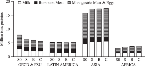
Livestock production change between 2000 and 2030 by region
Land Use and GHG Emissions
Cropland expansion is influenced by two opposite effects along the yield growth scenarios: a decrease in the acreage needed to produce the same quantities, and an increase in demand for feed crops as livestock shift toward mixed systems. In our baseline (B), 108 million hectares (Mha) of additional cropland enter production by 2030 compared to 2000 (figure 2). In the convergence scenario (C), 111 Mha of cropland would be spared, as the effect of crop intensification is greater than the increase in feed crop demand. On the other hand, 112 Mha and 289 Mha, respectively, of additional cropland would be required in scenarios (S) and (S0).
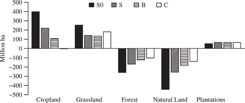
Land cover change between 2000 and 2030
More interestingly, crop yields are also found to have a large impact on grassland area. In the baseline (B), grasslands expand by 134 Mha between 2000–2030. But at 253 Mha, the expansion is almost twice that size under scenario (S0). However, the impact of crop yield growth on grassland area expansion is not monotonous. Under scenario (C), a further decrease in competition for land leading to a relative stagnation in the structure of livestock production systems, and growth of ruminant production in Asia and Africa, would lead to an increase in grassland area by 47 Mha compared to scenario (B).
The total agricultural land sparing under (B) as compared to (S0) is 409 Mha. This is 17% more than just cropland sparing alone due to higher yields, as it would be calculated outside the model by comparing the area needed to produce (B) scenario crop quantities with (S0) yields instead of (B) yields–349 Mha.
Total emissions from agriculture and land use change, calculated as annual averages for 2000–2030, range from 8,335 MtCO2-eq per year for scenario (S0) down to 6,444 MtCO2-eq for scenario (B), and 6,258 MtCO2-eq for scenario (C). The main source of emission reductions when crop yields increase lies in the slower conversion of forests and other natural vegetation to agriculture (figure 3). Intensification of livestock production and the reallocation of ruminant meat production leads to a slight decrease in livestock sector emissions in Latin America. The positive effect of intensification in Asia is more than compensated for by the reallocation of livestock production toward this region. In the crop sector, N2O emissions from crop intensification increase due to higher fertilizer use. This is compensated for in Asia by lower CH4 emissions from rice cultivation, given that a smaller area is used to grow the same production.
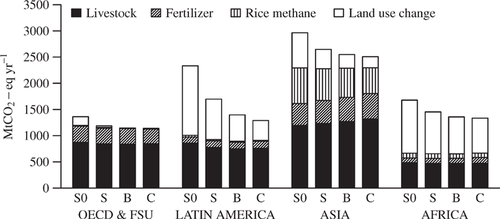
GHG emissions from agriculture and land use change as annual average, 2000-2030
Crop Yield Increase as a Mitigation Option
We have observed that increases in crop yields lead to the reduction of GHG emissions from land use and the agricultural sector of 1,351, 1,891, and 2,077 MtCO2-eq per year by 2030 for scenarios (S), (B), and (C), respectively, when compared with scenario (S0). To evaluate the cost efficiency of mitigating GHG emissions through productivity increases versus a carbon price policy, we put these abatement levels into perspective with a marginal abatement cost curve (MACC) calculated for scenario (S0) in GLOBIOM (figure 4). The MACC obtained is relatively flat up to 1,000 MtCO2-eq, where most of the cheap emission reductions through avoided land use change are realized; after this point, there is more and more demand for abatement in the agricultural sector, but this is expensive, as final consumption is kept at the baseline (B) level.
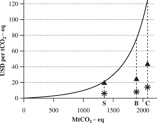
Marginal abatement cost curve for agriculture and land use change under scenario (S0)-plain line, and abatement levels with required R&D investments for scenarios (S), (B), and (C) (Land cover carbon density: high=asterisks, low=triangles)
A rough estimate of the research and development (R&D) investments necessary to attain yield growth levels corresponding to scenarios (S), (B), and (C) has been made following the methodology proposed by Burney, Davis, and Lobell (2010). The unit costs based on our results are represented by triangles in figure 4. These values indicate that the role of crop yield growth as a cost-efficient mitigation option increases with the level of the mitigation target. At the level of emission reductions resulting from scenario (S), the R&D investments needed to move from (S0) yields to (S) yields, and the carbon price sufficient to reach this mitigation level under the (S0) scenario would be roughly the same, that is, U.S. $20 per tCO2-eq. However, the carbon price necessary to achieve the GHG emission reductions corresponding to the difference between scenarios (S0) and (B) would be three times higher than the adequate R&D investment, that is, U.S. $75 per tCO2-eq versus US $25 per tCO2-eq.
Our results show the necessary R&D investment numbers to be substantially higher than those obtained by Burney, Davis, and Lobell (2010). This can be traced back to differences in assumptions about the carbon density of converted land. The necessary R&D investment corresponding to the average land cover carbon density considered by Burney, Davis, and Lobell (2010) is depicted in figure 4 by asterisks. As applying their carbon densities to GLOBIOM would also shift the MACC down, it is likely that the relative efficiency of carbon price versus yield growth policies at the different abatement levels would be unaffected by this assumption.
Conclusion
Crop yield development will play a critical role in future land use dynamics. Indeed, it will determine the requirements for additional cropland, and also have a strong impact on grassland expansion. We have illustrated that compared with yield stagnation, maintaining past trends in crop yield growth would save 290 Mha of cropland and avoid additional expansion of about 120 Mha of grassland by 2030. Our results suggest that failing to take into account the effects of livestock sector dynamics and the corresponding grassland requirements when assessing the effect on land sparing of increasing crop yield may lead to significant inaccuracy–a difference of 17% in our example.
With respect to GHG emissions, we show that by 2030 these would be lower by more than 2 GtCO2-eq per year if crop yields grew according to the past trends as compared to yield stagnation. Crop yield growth also seems to be a cost efficient way of abating GHGs, as the estimated R&D cost involved would be about U.S. $25 per tCO2-eq, while the marginal cost of reaching this target with stagnating yields would be U.S. $75 per tCO2-eq. However, to be effective as a mitigation option, crop yield increases need to be accompanied by policies that prevent further expansion of consumption in rich countries in order to avoid the potential rebound effects illustrated by Choi et al. (2011).
Overall, policies and investments targeting crop yield enhancement should be an important priority for the future of agricultural development (Herrero et al. 2010). Such measures could help to fight food insecurity, while at the same time contributing to climate change mitigation at a cost that is competitive with other mitigation strategies.


