Analysis of cosmic microwave background data on an incomplete sky

The spherical harmonics form a complete set of orthonormal basis functions over the entire sphere. They are most commonly defined as complex functions (e.g. Landau & Lifshitz 1976; Brink & Satchler 1993), but it is more convenient to use real harmonics in this application. Adapting the notation of Górski (1994), the real spherical harmonics are given by

where l≥0 and |m|≤l and

((A2))

implying that . For 0≤m≤l and −1≤x≤1 the normalized associated Legendre functions are defined by

((A3))

Hence 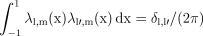. Under the same conditions the (unnormalized) associated Legendre functions are given by⁵

((A4))

with the Legendre polynomials given by

((A5))

A real field on the sphere, a(r^), can be expanded in terms of spherical harmonic coefficients, given by

This can be inverted to give

((A7))

provided that l_max→∞, due to the orthonormality of the spherical harmonics on the full sphere:

If a finite l_max is used this inversion is no longer possible for general a(r^), although it does still hold for band-limited functions.⁶

Whilst the two indices l and m have quite distinct interpretations, it is convenient to combine them into a single index, i, which allows the definition of vectors Y(r^)=Y_i(l,m)(r^) and a=a_i(l,m). Two obvious indexing schemes present themselves: grouping in l and m. The first, as introduced by Górski (1994), is natural for power spectrum estimation and very simple:

The two ‘inverses’ of this relationship are

and

The second choice of ordering is useful in cases of azimuthal symmetry in which the orthogonality expressed in equation (A2) is maintained, and grouping in m is achieved by defining

((A12))

The ‘inverses’ in this case are given by

((A13))

and

((A14))

Other indexing schemes have been used in the more specific case of simulated Planck data-sets in which the sky coverage is periodic in azimuth (van Leeuwen, private communication), but are beyond the scope of this paper.

In Section 2.3 integrals of the form

((B1))

arose; here the λ_l,m(x) are the normalised associated Ledengre functions, defined in equation (A3), and m is assumed to be non-negative. These integrals can be evaluated quickly and accurately using a combination of closed formulæ and recursion relations.

The associated Legendre functions, P_l,m(x) (defined in equation A4), are solutions of the ordinary differential equation (e.g. Arfken 1985)

((B2))

Multiplying this equation by P_l′,m(x) and integrating (from x₁ to x₂) by parts twice yields

((B3))

This is a reflection of the standard result that integrals of solutions of a self-adjoint differential equation (as equation B2 is) can be expressed as boundary terms (e.g. Arfken 1985). The derivatives in equation (B2) can be removed by using the standard recursion relationship (e.g. Gradshteyn & Ryzhik 2000)

((B4))

to yield, for l≠l′,

((B5))

Note that the first term must be omitted if l′=m and that the third term must be omitted if l=m; these Legendre functions are implicitly zero from equation (A4). Finally, this can be normalized according to equation (A3), giving

((B6))

An alternative derivation of this result was presented by Wandelt et al. (2001); it is also in principle equivalent to equation (13) in section 5.9 of Varshalovich, Moskalev & Khersonskii (1988), but their application of equation (B4) is in error.

For the case l=l′, a recursion relation is required, starting with l=m. Combining equations (A3) and (A4),

((B7))

where n!!=1×3×⋯×(n−2)×n for odd n. Integrating by parts and using equation (B7) again gives

((B8))

Moving to l=m+1, the standard relationship (e.g. Gradshteyn & Ryzhik 2000) that

combines with equation (B7) to give

((B10))

where the first term is given in equation (B8).

The last step is to derive a recursion relation relating I_l,l,m(x₁,x₂) to I_{l−1,l−1,m}(x₁,x₂) and I_{l−2,l−2,m}(x₁,x₂). Equation (C22) of Wandelt et al. (2001) gives a four-term recursion to obtain I_l,l′,m(x₁,x₂); it can be applied successively (once swapping l and l′) to obtain

((B11))

In summary, equation (B6) can be used to evaluate all I_l,l′,m(x₁,x₂) for which l≠l′, and equations (B8), (B10) and (B11) combine to give all I_l,l,m(x₁,x₂) recursively.

All the cosmological information encoded in the CMB is expected to be contained in the l≥2 modes; the l=0 mode in an isotropic universe can be normalised arbitrarily and the l=1 modes can be set to zero by adopting an appropriate reference frame. None the less, observations of the microwave sky will yield non-zero monopole and dipole values for a number of reasons (e.g. the observer's motion; Galactic emission; extragalactic point sources). Hence these low-order modes must be included in the analysis of CMB data, but should be kept separate from the cosmological modes, as is naturally the case if spherical harmonic coefficients are used to describe the data. It is also important to note that the properties of the basis functions themselves are unimportant – the essential requirement is that only four of the cut-sky harmonic coefficients contain information on the unwanted modes.

The method of orthogonalization summarized in equations (11), (12) and (14) does not explicitly impose any particular structure on the conversion matrix, A (which relates harmonic coefficients on the incomplete sphere to those on the full sphere by a′=A^Ta;equation 24). The non-cosmological modes are kept separate from the cosmological modes if the first four columns of A^T have only zeros from the fifth row on, assuming the full-sky harmonic coefficients are indexed using l-ordering (Appendix A). This is achieved naturally if A^T is constructed to be upper triangular, as in the case of the Cholesky decomposition described in Section 2.2.1. The other decomposition methods discussed in Section 2.2 do not share this property, and so the resultant conversion matrices must be adjusted explicitly.

One way of achieving this is to use a partial Householder transform (e.g. Press et al. 1992). The last i′_max−i elements of the ith column of a general i′_max×i_max matrix can be set to zero by the transformation M′=P_iM, with the orthogonal Householder matrix defined by

((C1))

where m_i is given by

((C2))

and i≤min(i′_max,i_max) is assumed. Provided that the Householder matrix applied to B is that generated from A^T, the transformations A′^T=P_iA^T and B′=P_iB leave equations (12) and (14) unaffected as P_i is orthogonal by construction. Applying P₁, P₂, P₃ and then P₄ to the successively updated A^T ensures that the l=0 and l=1 modes influence only the first four cut-sky harmonic coefficients, as required. This procedure could be continued, moving A^T successively closer to upper triangular form, although this cannot be achieved in full as A^T has more columns than rows.

Special mention must be made of the constant latitude cut case, the symmetry of which can only be utilized if the spherical harmonics are indexed using m-ordering (Appendix A). In this case only the m=0 and m=±1 blocks have any contribution from the monopole or dipole, and each can be treated separately. Further, the ordering within these blocks is such that the non-cosmological modes are in the first rows, and so the above algorithm can be applied to each of three blocks as is. The only slight inconvenience is that it is no longer the first four cut-sky modes that contain the non-cosmological information, and the relevant modes must be flagged explicitly.

This paper has been typeset from a tex/latex file prepared by the author.