Observability of the ambient conditions in model-based estimation for wind farm control: A focus on static models

1 INTRODUCTION

The European Wind Energy Association (EWEA) predicts the amount of installed wind energy to increase from 106 GW in 2012 to 735 GW in 2050, which at that point should provide for about of the European Union's electricity demand.1 The success of wind energy largely relies on its financial competitiveness with other renewable and nonrenewable sources. Control plays an invaluable role in this matter. In the past, the focus of control research has been on wind turbine control. Recently, the interest has largely shifted towards wind farm control (WFC), in which multiple turbines inside a wind farm are coordinated together to improve their combined energy yield.2 WFC addresses the issue of wakes, which are slower and more turbulent pockets of air that form behind a wind turbine as energy is extracted. Wake formation has led up to an estimated loss in the annual energy yield of the closely spaced Lillgrund offshore wind farm at the coast of Sweden compared WITH an idealized situation without wake formation.3 The underlying concept of WFC is to influence the wake such that it has a smaller impact on downstream turbines. A popular approach in the literature is yaw-based wake steering, in which the wake position is shifted laterally by purposely operating an upstream turbine at a yaw misalignment. Recent studies have shown the potential of yaw-based wake steering for wind farm power maximization in high-fidelity simulation,4 wind tunnel experiments,5 and field tests under dynamic inflow conditions.6-8 These publications suggest an increase in the annual energy yield in the order of 1% and situational increases of up to 20% for certain wind farms under particular inflow conditions that cause large wake losses.

The wake losses and therefore the amount of yaw misalignment that maximizes the energy yield is highly dependent on the wind direction, wind speed, and turbulence intensity of the incoming wind field.3 As these atmospheric conditions constantly change, so do the optimal yaw angles. Typically, a simplified (“surrogate”) model of the flow and turbine dynamics is leveraged to calculate the optimal yaw angles.9 However, due to the complicated flow behavior at a range of temporal and spatial scales, no surrogate model exists that is accurate for all the different atmospheric conditions a wind farm may encounter. For this reason, closed-loop control solutions are becoming increasingly popular in the literature.2 The underlying idea of this closed-loop control framework is that the surrogate wind farm model is continuously adapted such that it accurately and consistently predicts the wind farm behavior.

The closed-loop WFC framework is shown in Figure 1. This framework consists of three components, namely, (a) a surrogate wind farm model, (b) a model adaptation algorithm, and (c) a control setpoint optimization algorithm. Surrogate wind farm models can typically be separated into static and dynamic models. These model types attempt to predict the minute-averaged and the second-to-second flow and turbine behavior, respectively. The purpose of the model adaptation algorithm is to modify parameters inside the surrogate model such that it can accurately predict the wake interactions inside the wind farm, which includes the freestream wind speed and wind direction. Finally, an optimization algorithm is necessary to determine an optimal control policy such that a particular wind farm objective is achieved, eg, maximization of the wind farm power production. The focus in this article is on the model adaptation algorithm; the interested reader is referred to the survey by Boersma et al2 for more information on surrogate models and optimization algorithms.

The body of literature on real-time model adaptation for WFC is scarce. Most WFC literature has focused on setpoint optimization and model development.2 This goes paired with the fact that most WFC algorithms in the literature have been tested under quasi-steady ambient conditions, meaning that the mean wind speed, wind direction, and turbulence intensity were time invariant. This holds for both numerical simulations4 and real-world scaled experiments.5, 10 This limits the applicability of such algorithms, as the experiments do not sufficiently represent the real-world fluctations in the atmosphere.

A handful of articles in the literature is concerned with the estimation of atmospheric conditions and model adaptation for WFC. Annoni et al11 proposed a model-free algorithm to estimate the wind direction inside a wind farm using the wind vane measurements of different turbines and obtaining a consensus on the most probable value. Doekemeijer et al12 proposed a method to estimate the freestream conditions by a model inversion approach using the time-averaged turbine power measurements and a static surrogate model assuming the wind direction is known, which is comparable with the idea coined by Gebraad et al.4 Furthermore, Gebraad et al13 synthesized a Kalman filter for their dynamic surrogate model, which uses the turbine power measurements to estimate the flow field inside the wind farm. The adapted surrogate model was able to accurately predict the wind farm dynamics, though the wind direction was constant and assumed to be known. Similarly, Doekemeijer et al14 used a dynamic surrogate model with an ensemble Kalman filter to estimate the flow field and turbulence intensity using turbine power measurements. High-fidelity simulations showed that the algorithm was able to successfully reconstruct the dynamic wind field for a two-turbine and a nine-turbine wind farm. However, also in this work, the wind direction was assumed known. Further, Shapiro et al15 synthesized and evaluated a WFC solution assuming a constant wind direction. Besides the estimation of the ambient conditions, Bottasso and Schreiber16 attempt to estimate several model tuning parameters to improve the accuracy of the surrogate model.

This article is organized as follows. The surrogate model used in this work is presented in Section 2. The issue of estimation and a novel quantitative measure of observability is presented in Section 3. Simulation results are shown in Section 4, and the article is concluded in Section 5.

2 SURROGATE MODEL: FLORIS

The surrogate model used in this work is referred to as the “FLOw Redirection and Induction in Steady-state” (FLORIS) model.9 This model predicts the time-averaged power capture of each turbine and the time-averaged three-dimensional flow field for a wind farm under a specified set of inflow conditions. The timescale of FLORIS is on the order of minutes. A schematic overview of the types of inputs and outputs to the FLORIS model is shown in Figure 2. Fundamentally, FLORIS combines several submodels from the literature. The main components of FLORIS used in this article are described in the remainder of this section.

Firstly, FLORIS includes the single-turbine wake model from Bastankhah and Porté-Agel,17 which predicts the time-averaged three-dimensional wind field behind a turbine. Secondly, the turbine-induced turbulence is calculated using an empirical function proposed by Crespo and Hernández.18 Thirdly, the wind field under multiple overlapping wakes is calculated through a sum-of-squared-deficits law as proposed by Katic et al.19 Fourthly, the power production of each turbine is calculated using the rotor-effective wind speed and the nondimensional power coefficient , as

(1)

where is the air density, is the rotor swept area, is the spatially averaged inflow wind speed at turbine , and is the yaw angle of the turbine relative to the incoming wind. The nondimensional power and thrust coefficients, and , can be derived using actuator disk theory for aligned inflow ( ). Alternatively, the nondimensional power and thrust coefficients can be calculated using an aero-elastic turbine simulation model for various wind speeds (and yaw misalignment angles) such as OpenFAST20 or Bladed. A common expression modeling the effect of a yaw misalignment on the turbine power production is4

(2)

where has a typical value of to , depending on the wind turbine.

The results of an arbitrary wind farm simulation with two 10-MW turbines21 is shown in Figure 3. The computational cost for a single FLORIS run is 10 millisecond to 1 second, depending on the number of turbines in the wind farm. FLORIS has shown a good match with results from high-fidelity simulations,12 wind tunnel experiments,22 and field tests.8, 23 Furthermore, the variant presented in this article has fewer tuning parameters than a comparable model proposed in Gebraad et al.4 For a more detailed, mathematical description of the model, the reader is referred to its related literature. Note that the results that will be presented in this article are not limited to FLORIS and can straightforwardly be reproduced with other static surrogate models.

3 METHODOLOGY: INTRODUCING A MEASURE OF OBSERVABILITY

The model adaptation solution of a WFC algorithm is not guaranteed to result in satisfactory performance. There has to be sufficient information in the wind farm measurements to correctly determine the ambient conditions. Hence, an observability analysis provides useful insight before the implementation of such a control algorithm. The traditional definition of observability refers to dynamical systems; a system is observable if the initial conditions and the time series of the system states can be reconstructed from a time series of the system output signals. As FLORIS is a static model, such a notion does not apply. Therefore, a static observability notion is defined as being true for a situation when the initial conditions can be reconstructed from the system output signals. In this section, a mathematical definition of this observability is introduced for the control framework presented in Figure 1.

3.1 Cost function in estimation

Generally, a simplistic, heuristic approach is used to determine the prevailing ambient conditions inside the wind farm. However, the reliability of such methods vary, the literature on them is scarce, and these methods are limited in their accuracy. Rather, in this work, a surrogate wind farm model is leveraged in a sensor fusion approach for the estimation of the ambient conditions.

In this work, the freestream wind speed, wind direction, and turbulence intensity are estimated using the readily available measurements of each turbine. For example, consider a cost function that minimizes the error with the time-averaged power measurements of each turbine, as

(3)

with the number of turbines, and , , and being the freestream wind direction, wind speed, and turbulence intensity as evaluated in FLORIS, respectively. 1Using this cost function for model adaptation, the idea is that values for , , and are found such that the error between the measured turbine power signals and what is predicted by FLORIS for these conditions is minimized. The cost function shown in Equation 3 was used for model adaptation in Doekemeijer et al12 assuming was known a priori, which allowed the successful estimation of and . However, only using the turbine power measurements may lead to situations in which the true ambient conditions cannot be reconstructed accurately. For example, consider the case in which all turbines inside the wind farm are operating in above-rated conditions. All turbines are then generating their rated power, and one cannot distinguish different above-rated wind speeds from one another. To resolve this issue, one can include the wind speed estimates from a local turbine wind speed estimator24, 25 in the cost function. This term is denoted by , given as

(4)

where is the measurement of the local wind speed estimator of turbine , and is what FLORIS predicts the local wind speed to be at turbine for the hypothesized wind conditions , , and . Note that the inflow wind speed at a turbine in FLORIS, denoted by , is the freestream-equivalent wind speed at that turbine under zero yaw misalignment. Thus, the effects of a yaw misalignment of turbine are not accounted for in this signal. However, in practice, a typical local turbine wind speed estimator provides a freestream-equivalent wind speed using the turbine power signal under the assumption of zero yaw misalignment. To account for the situation in which a turbine is misaligned with the flow, one can model as

(5)

in order to match the signal definition from the local wind speed estimator, . Finally, one can combine and into cost function , as

(6)

where and are weighing terms. Using the cost function defined in Equation 6, difficult situations may arise when trying to estimate , , and . For example, if there is no wake interaction, one cannot estimate the freestream turbulence intensity, as the effects of have no correlation with (ie, impact on) the measured signals. Moreover, issues may arise concerning the estimation of , as demonstrated in Figure 4.

In this situation, and yield almost identical values for and , thereby making it impossible to distinguish these two situations using the measurements available.

To address the latter issue, local wind direction estimates of each turbine are included in the cost function, eg, using the filtered wind vane measurements.26 This term is modeled as , given by

(7)

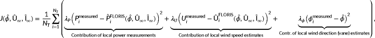
where is the filtered wind vane measurement of turbine and is the hypothesized wind direction in FLORIS. The complete cost function is now defined as

(8)

with a weighing term for the local wind direction estimates. This weighing term is to be chosen according to the relative measurement noise and bias in the wind vane measurements, and could vary per turbine. The to-be-estimated quantities are , , and . Each of the three components includes a squared term to quadratically penalize mismatches between the surrogate model and sensor measurements. The situation of Figure 4 becomes increasingly better conditioned as the contribution of the wind vane measurements increases, as visualized in Figure 5.

Thus, it is clear that local wind speed measurements (to deal with above-rated wind speeds), wind direction measurements (to deal with situations as exemplified in Figure 4), and wake interaction (to enable correlation between and the measurements) are required to promote observability of the freestream conditions over the full range of operation. When multiple minima exist at a notable distance from the true solution (in the example case of Figures 4 and 5, this would be , with ), the ambient conditions cannot be reliably estimated, and the situation becomes unobservable. 2

However, while it is clear that particular situations are unobservable, a quantitative measure is still required to determine the degree of unobservability. For example, is the situation in Figure 5 with “observable enough” to uniquely determine the ambient conditions? To answer such questions, a quantitative measure of unobservability for static models is introduced in the next section.

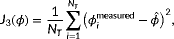
3.2 A quantitative measure for unobservability

With the cost function defined, a quantitative measure on the degree of observability of a particular situation is defined. With “situation,” we imply a particular wind farm layout, the true ambient conditions and a specific choice of the regularization terms , , and . The main contribution of this paper is the introduction of such a mathematical notion for observability. The observability of a particular situation is defined as

(9)

(10)

with as defined in Equation 8, , , and denoting normalization terms, and , , and being thresholds. Further, , , and denote the difference between the true and hypothesized ambient conditions, respectively. In the remainder of this section, the working principle will be explained.

The function is defined such that critical points (low cost , far away from the true solution) have a low value (less observable—hard to tell apart from the true solution), while situations in which the cost is high yields a high value (more observable—easier to distinguish from the true solution). Furthermore, the threshold terms are present to ensure that any value estimated close enough to the true optimum does not “endanger” the observability. A more elaborate discussion on these thresholds can be found in Appendix Appendix A.

Figure 6 demonstrates how the observability is calculated for the example situation discussed in Section 3.1. Note that this is not necessarily a realistic scenario, but rather is discussed to provide insight into the method. The function is derived from the cost function following Equation 10. The cost function has two minima: one at and one at , indicating that there are two hypothetical wind directions that produce near-identical turbine power signals. This leads to a low observability.

Note that the measured quantities in are taken as the values from the surrogate model (FLORIS) with the true ambient conditions, thus assuming a perfect model of the system. In reality, this will not hold, and the work herein presents an idealized case (theoretical upper bound) of observability.

Finally, with a measure for observability defined, we can determine and analyze the observability of a particular wind farm for a certain wind direction, wind speed, and turbulence intensity. The process is as follows.

1. Firstly, we evaluate the degree of observability of a single situation at a time. With a situation, we imply a wind farm subjected to a certain ambient inflow, giving us a certain set of measurements. For example, continuing the example two-turbine wind farm of Section 3.1, the observability for this wind farm is investigated at a true freestream wind speed of 7.0 m s , a freestream wind direction of , and a turbulence intensity of . Referring back to Figure 4, our measurements would be
   (11)
   (12)
   (13)
   The measurement vectors contain two entries, for turbines 1 and 2, respectively. In this simulation, the turbines are assumed to be aligned with the inflow wind direction; .
2. Secondly, we now assume that we do not know what the ambient conditions generated these measurements. This represents our estimation step. With this set of measurements, the cost function of Equation 8 is calculated for a range of hypothetical (tested) ambient conditions. For this example, the estimation algorithm is limited to the estimation of and . The (two-dimensional) cost function is evaluated over the following ranges:
   (14)
   (15)
   (16)
   If is additionally to be estimated, the (three-dimensional) cost function is also evaluated over the following range for :
   (17)
   Furthermore, the turbine yaw angles are fixed in the inertial frame and assumed to be known a priori in the cost function evaluations. Thus, if the cost function is evaluated for , then .
3. Finally, we check whether our estimation algorithm was successful. A two-dimensional (for ) or three-dimensional (for ) cost matrix is obtained following Equation 8, from which is calculated following Equation 10. The degree of observability is the minimum value of , being a positive real number.

The degree of observability can be calculated for a range of true wind directions following the process described above and displayed in a single picture. The results of such an observability analysis assuming only power measurements are available ( , and ) are shown in Figure 7 for a six-turbine wind farm. Note that and are zero to provide insight into the results. In a practical WFC implementation, one would opt for and , if these measurements are available.

Each of the two radial plots shown in Figure 7 represents the degrees of observability for 61 different wind directions. There is one degree of observability defined for each true wind direction, plotted as a particular color across the polar axis. This thus indicates the estimability of and for this true wind direction. For each of the 61 true wind directions, a two-dimensional cost function was calculated over the variables and  m s . Then, was taken to be the lowest value of , being the degree of observability for this true wind direction, true wind speed, true turbulence intensity, wind farm layout, and with and being the to-be-estimated parameters. We refer to this as the degree of observability for this particular situation.

Figure 7 clearly shows that the and can only be estimated for a narrow range of true wind directions when only power measurements are available. This makes sense, since there is only wake interaction for a small range of wind directions. Without wake interaction, one cannot distinguish, for example, between the case where all turbines operate under a yaw misalignment and a higher inflow wind speed, from the case where all turbines operate without a yaw misalignment and a lower inflow wind speed. Furthermore, an interesting difference between the observability plot for a true wind speed of 6.5 and 9.0 m s is the degree of observability at the true wind directions of and . This is because of the fact that the downstream turbines operate below cut-in wind speed for the 6.5 m s case at these wind directions due to the close spacing and the wake effects. As these downstream turbines do not generate any power, their signals hold little information. For the 9.0 m s case, all turbines operate above cut-in wind speed, and thus, these power signals contain more information about the flow.

The methodology presented in this section serve for explanation purposes, and the cases becomes more interesting when considering more complicated farm layouts, various combinations of wind vane and wind speed measurements, and the inclusion of turbulence intensity estimation. This is the focus of the next section.

4 A COMPREHENSIVE OBSERVABILITY ANALYSIS FOR THREE WIND FARM LAYOUTS

The observability of the ambient conditions is investigated in this section for three different wind farm layouts, namely, two symmetrical wind farms and one asymmetrical wind farm. The layouts are shown in Figure 8. The asymmetrical eight-turbine wind farm is an interesting configuration, as there is more unique wake interaction situations in this layout. This reduces the issues with symmetry previously demonstrated in Figure 4 compared with symmetrical wind farm layouts.

For each topology, the observability is calculated for situations, namely, for 61 wind directions , 4 levels of turbulence intensity , and four wind speeds  m s , of which the latter wind speed is above rated. Thus, for each of these 976 conditions, a multidimensional cost function is set up, and the most critical situation is determined following Equation 10, upon which the observability for this situation is calculated using Equation 9. The parameters therein are shown in Table B1.

This section is separated in two parts. In Section 4.1, the observability of the various situations is assessed under the assumption that the freestream turbulence intensity is known a priori. This simplifies the estimation problem and requires less information to be extracted from the measurements at hand. However, neglecting the estimation of is expected to significantly worsen the accuracy of the surrogate model in a practical WFC algorithm. Hence, the observability with the inclusion of is presented in Section 4.2.

4.1 Estimating and under perfect knowledge of

First, the observability of various situations under the assumption that the turbulence intensity is known, , is looked into. The range over which each particular cost function is calculated is and  m s . The discretization of these parameters were tuned for convergence, such that the solutions no longer notably change at a higher precision. The range of these parameters is chosen to resemble the typical prior knowledge one has about the true ambient conditions in such an estimation problem.

4.1.1 Redundancy in the cost function: Power and wind speed estimates

One important notion in the cost function shown in Equation 8 is that the local wind speed estimates and the turbine power signals carry duplicate information. Specifically, as the local wind speed estimators rely on the turbine power signal, the turbine power measurements theoretically add no information to the cost function that is not already included in the wind speed estimator signals. To validate this, an observability analysis is performed for the six-turbine wind farm under and various values for and . The results are shown in Figure 9.

From this figure, one can immediately see that situations in which all turbines are in above-rated operation are unobservable when (top-right subplot). This subplot shows some observability when the turbulence intensity is low and the wake interactions are deep, such that one or multiple downstream turbines are operating below rated conditions. Furthermore, turbine power measurements do not add anything to the observability compared with the wind speed estimates. Note that the observability plots are not identical for below-rated conditions as power is cubically related to the wind speed, , and thus, the observability is spread slightly differently within the radial plots. Though, the trends are identical. Hence, in the remainder of this work, .

An important remark is that a different surrogate model, eg, one that directly correlates the upstream turbulence intensity with the upstream turbine power production, may provide a higher degree of observability from the same power measurements. Currently, such a correlation is not present in FLORIS.

4.1.2 Using exclusively wind speed estimator measurements ( , , )

Here, the situation with solely wind speed measurements available is investigated; and . This is comparable with the estimation framework applied in previous work,12 in which wind vane measurements were not assumed to be available. This is a particularly difficult problem, as previous results from Section 3 suggest. In the remainder of this section, all three wind farm layouts will be addressed. The observability roses are shown in Figure 10.

A number of observations can be made from Figure 10. Firstly, for the two-turbine wind farm, it is clear that the wind direction and wind speed can only be estimated accurately for a narrow range of wind directions—specifically, in which there is sufficient wake interaction. Theoretically, the can always be reconstructed from the wind speed estimate of the upstream turbine, and the upstream turbine can be distinguished if there is wake interaction: it is the turbine with the highest power signal. The wind direction can then be estimated by looking at the quantity of wake losses at the downstream turbine. However, this may lead to situations in which two hypothesized wind directions lead to a near-identical inflow wind speed , as was seen previously in Figure 4.

Secondly, for the six-turbine wind farm, it can be seen that this topology has more wake interaction than the two-turbine wind farm and thus has an increased observability for many situations. However, there are still situations with little to no wake interaction which are unobservable. Note that the radial plots for both the two-turbine wind farm and the six-turbine wind farm are radially symmetrical, as the topologies are also radially symmetrical.

Thirdly, for the eight-turbine wind farm, one can directly see that observability greatly increases due to many more unique wake interaction between turbines. With all topologies, generally, it is noted that a higher atmospheric turbulence leads to a lower observability. Specifically, the turbulence intensity reduces the wake interaction with downstream turbines. The results from Figure 10 show that and can only be reconstructed for particular situations, and thus, care has to be taken in such estimation algorithms and related WFC algorithms. The next section shows the estimability of and with the inclusion of wind vane measurements.

4.1.3 Using local wind speed and wind direction estimates ( , , )

By including local estimates of the wind direction, , one can attain observability for all situations, as shown in Figure 11. Now, one assumes both wind speed measurements and wind vane measurements to be available.

It is clear to see that all the necessary information is contained in the measurements available for the estimation of and : all situations appear observable. Observability is guaranteed due to the availability of local wind speed and wind direction measurements, which are quantities directly derived from the ambient wind speed, ambient wind direction, and the wake interactions. Note that there are some variations within the radial circle, which are both due to physical effects such as more or less wake interaction and due to fact that the search space of the cost function ( , , ) is discretized at a finite resolution.

The tools presented in this work may prove useful to find a balanced trade-off in the cost function between the contributions from various measurement sources. However, even with an accurate estimation of and , significant model discrepancies may remain. The freestream turbulence intensity has a relatively large impact on the optimal turbine setpoints for wake steering, as it has a direct relationship to the degree of wake recovery. Hence, the estimation of is a necessity in reliable WF algorithms. In the next section, the estimation of is incorporated into the observability analysis.

4.2 The full estimation problem: Estimating , , and

While observability for all situations was shown in Section 4.1.3, a compromising assumption was made that the freestream turbulence intensity was known. In reality, this is not a realistic assumption and must be estimated together with and . The observability when estimating , , and is shown in Figure 12, where .

Several observations can be made. Firstly, one can directly see that the observability significantly reduces for a large range of conditions compared with only the estimation of and . For the two-turbine case, observability only remains for the narrow window of wind directions in which there is wake interaction. This can be explained by the fact that the measurements provide direct information on and , while the estimation of is enabled through inversion of the surrogate model and the usage of the local wind speed measurement at the downstream turbine. This only applies when wake interaction is present.

Secondly, observability is reduced in the six-turbine case compared with Figure 11, yet observability remains more widespread than the two-turbine case. More wake interaction and multiple-wake interaction leads to the fact that the turbine power signals are more sensitive to the freestream turbulence and thus yield a higher observability than the two-turbine case. Additionally, while a higher turbulence intensity leads to additional wake recovery, it also leads to wider wakes which can impact a downstream turbine where it would not for lower turbulence intensities. These two effects have an opposite effect on the observability, and hence observability does not uniformly decrease with an increase in the freestream turbulence intensity.

Thirdly, the eight-turbine wind farm has the most observable situations from the three topologies. Due to the many unique wake interactions, the solutions become relatively sensitive to the freestream turbulence intensity, and the ambient conditions can be estimated for most conditions. Though, also in this wind farm, one can find several situations in which the freestream conditions cannot uniquely be reconstructed from the measurements available.

An important remark to make is that all results presented in this section ignore the possibility of other measurement sources. While this framework allows the inclusion of turbulence intensity measurements, this was not pursued here. Additionally, one may argue that temporal correlation of measurements would allow for additional information on the ambient conditions. This would require a dynamic mathematical model that correlates the ambient conditions and the turbine measurements and a state estimation algorithm such as a Kalman filter. This is out of the scope of this article.

Finally, recall that these results present an idealized case, in which there is no measurement noise, and the surrogate model is used to generate the measurements, implying that the surrogate model perfectly represents reality. None of these assumptions are valid in practice, and thus, the observability roses presented in this section will further diminish. Though, the results presented in this section are an useful step towards the synthesis of an algorithm that estimates the ambient conditions in a robust manner. The observability roses from Figure 12 provide a theoretical upper limit on the relative estimatibility of the ambient conditions , and from the measurements available. This can provide guidance in C algorithms on when to estimate certain parameters. Since and are always estimable according to Figure 11, the observability analysis presented in this section can be used to determine whether to estimate in addition to and . If the situation is observable enough (which is to be selected experimentally), the measurements should contain sufficient information to reliably estimate . If not, one can assume to be equal to its past value (since the turbulence intensity also does not change very rapidly in the field) and exclusively estimate and . This approach is currently being explored and will be published in future work.

5 CONCLUSIONS

Over the last years, the scientific community surrounding WFC has shown an increasing amount of interest towards the real-time estimation of the ambient conditions inside a wind farm. This ambient flow information is essential to the optimization of the turbine yaw angles for wake steering, which is currently the most popular methodology of WFC for power maximization. The degree of reconstructability of the ambient conditions highly depends on the meaurements available and the wind farm layout. For many situations, it is clear to see that the ambient conditions cannot be estimated. However, no quantitative measure exists to represent the degree of estimability of the ambient conditions. This paper addresses this scientific gap.

The main contribution of this paper is the introduction of a novel, mathematical definition for the observability of the ambient conditions. This measure describes how well the true ambient conditions can be distinguished from hypothesized ambient conditions through a model inversion approach for a particular set of measurements. This measure of observability is modular and can easily be extended with other measurement sources or other surrogate models. While a number of outcomes of this article may seem apparent, this theoretical framework provides the tools for extended analysis and a quantitative measure for the estimability of the inflow properties leveraging different measurement sources and surrogate models.

In several case studies, we show the usefulness of the proposed measure. Moreover, while information concerning the wind direction can be derived by looking at the turbine power signals and the inter-turbine wake interactions, the case studies presented show that there is a strong need for wind direction measurements for WFC to sufficiently cover observability for any topology and any ambient condition. Generally, situations in which there is sufficient wake interaction are observable, while situations with little to no wake interactions are unobservable. 3Furthermore, the mathematical framework supports the straightforward notion that local turbine power measurements provide no additional information compared with local wind speed estimates, implying that power measurements can be omitted from the cost function. 4Also, more complicated, unstructured wind farm layouts generally result in a higher observability as there are more unique wake interactions between turbines.

In general, even with local wind speed and wind direction information, one still cannot reconstruct the full set of ambient conditions (wind speed, wind direction, and turbulence intensity) for all conditions that a particular wind farm may encounter. Thus, before one may attempt to estimate the ambient conditions, one should consider whether the situation is observable in the first place. Using this information, one may condition their WFC algorithm to situations that are sufficiently observable. This aids in improving the reliability of WFC algorithms and thereby hopefully the willingness to adopt such algorithms by the industry.

Conflict of interest

The authors declare no potential conflict of interests.