Modeling membrane geometries implicitly in Rosetta

2.1 We added different implicit membrane geometries to RosettaMP

This substantial refactor was geared to achieve multiple goals: (1) adapting the current implicit membrane models for geometries that mimic micelles, bicelles, vesicles, membrane curvature, and double bilayers, (2) adapting the code interface to facilitate implementation of new geometries (e.g., lipidic cubic phases), (3) streamlining the current implementation by disentangling the pore from membrane geometries to be used independently and creating a membrane representation from a single, consistent implementation, thereby (4) minimizing code duplication, (5) improving testing, and (6) visualizing membrane geometries onto protein structures.

2.2 Previous implicit membranes in Rosetta only describe a flat membrane

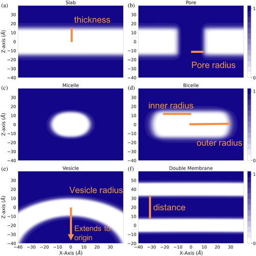
Mathematically, the membrane is modeled by a transition function that describes the transition from the aqueous environment to the hydrophobic environment of the membrane. Two transition functions had previously been implemented, one based on IMM1 and an adaptation to model different lipid compositions. Disregarding the pore, both transition functions score atoms based on their distance from the center of a membrane plane, meaning that the hydrophobicity at a specific position is only dependent on the depth in the membrane (z-coordinate). This creates the implicit slab membrane (Figure 1a).

2.3 Expanding beyond flat membranes through implementation of mathematical representations of desired geometries

To model different geometries, transition functions must depend on the distance to the membrane center in more than one dimension. The pore was the first adaptation that introduced a three-dimensional dependence (Figure 1b). In order to create an ellipsoid geometry similar to micelles and bicelles, we created a functional form that combines the slab transition function (He et al., 2013) with a function that depends on the distance to the center of the ellipsoid (Figure 1c,d). Although micelles and bicelles have different chemical and physical properties, we use the same function to describe their shape whereas the micelle is a special case of the bicelle with an inner radius of the ellipsoid (Figure 1d) just large enough to surround the transmembrane region of the protein. To model a curved membrane such as a vesicle, we model the membrane as a sphere with the sphere's center at (0, 0, −R), with R being the radius of the sphere or vesicle. The protein is embedded in the membrane around the origin (0, 0, 0) which is at the center of the membrane. Therefore, location of the membrane residue used in the RosettaMP framework, which stores information about the implicit membrane position and orientation, remains the same with a structure already transformed into membrane coordinates using the RosettaMP framework (Alford et al., 2015). The vesicle concept is extended to describe two membranes by a double vesicle (two concentric spheres) that, with a large radius, represent two essentially flat membranes (Figure 1f). Detailed descriptions of equations and parameters can be found in Section 5.

2.4 Code design ensures current and new geometries are compatible across membrane energy functions

To achieve our goal of generalizability across score functions and simplify the implementation of new geometries, we introduced an abstract base class into the RosettaMP framework that all other membrane geometry classes are derived from (Figure S1). By defining pure virtual functions within the MembraneGeometry base class, we ensure that all derived classes (or new geometries) define the transition function and the derivative of the transition function for that geometry. Functions used across different geometry classes are defined in the MembraneGeometry base class to decrease code duplication. For example, the functions for describing the pore are now defined in the MembraneGeometry class where they can be combined with different transition functions and geometries while keeping the equations describing the pore environment the same as originally implemented (Alford et al., 2020). Implementation details, function definitions, and score terms that depend on them, can be found in Section 5. This implementation ensures that new geometries can be implemented by solely creating a class and updating options for setting the new geometry without updating each individual score term that depends on the transition function. This also allows for geometries to be used across score terms without the need to define the geometries or transition functions separately for each score term, including the equations describing the pore. Therefore, membrane-dependent score terms that use a transition function implemented before the pore can utilize the pore model as well.

2.5 Optimized code design allows for integrating membrane geometries into different applications

Implementation of the membrane geometries following the same object oriented design principles used in the RosettaMP framework allows for use in any application accessible to the RosettaMP framework (Alford et al., 2015), including but not limited to design, refinement, and protein–protein docking. This implementation also ensures a consistent user interface with the same command line options for setting geometry parameters across applications. The membrane geometries are also accessible through the different Rosetta scripting interfaces, including RosettaScripts (Fleishman et al., 2011) and PyRosetta (Chaudhury et al., 2010).

2.6 New implementation decouples pore model from energy functions, as tested for design

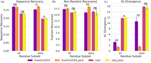
Alford et al. described an improvement in protein design using their newly developed energy function, franklin2019, compared to previous membrane energy functions (Alford et al., 2020). However, it was not clear if these improvements came from the new energy function, from the inclusion of the pore, or a combination of the two. This could not be tested because the pore was incompatible with older membrane energy functions. Our reimplementation of the pore function into the MembraneGeometry class allows for its use across applications and energy functions. Therefore, we are able to test protein design including the pore for both energy functions, mpframework2012 and franklin2019. We used an established membrane protein design benchmark set to test where this improvement comes from (Alford et al., 2021). The test uses three different metrics to describe performance: (Alford et al., 2020) sequence recovery is the fraction of native residues recovered after design over all designable positions. (Alford et al., 2015) non-random recovery of individual amino acids, where the recovery rate for each amino acid is calculated relative to the background probability of randomly guessing the native amino acid (1/20). (Alford et al., 2021) The Kullback–Leibler (KL) divergence measures how different distributions of designed amino acids are compared to native distributions. The design test done on the subset of proteins from the dataset that contain a pore to highlight the effect of accounting for an aqueous pore. The design protocol was run with six different energy function conditions: mpframework2012 without the pore included, mpframework2012 with the pore, franklin2019 without the pore, franklin2019 with the pore, ref2015_memb (Weinstein et al., 2019), and ref2015 (Figures 2 and S2). When analyzing all residues in each protein, franklin2019 outperforms the mpframework2012 energy function with respect to all three metrics. Inclusion of the pore in either franklin2019 or mpframework2012 score functions does not improve the sequence recovery or non-random recovery when looking at all residues, but improvement in the KL-divergence is observed for franklin2019 (Figure 2). The franklin2019 with the pore outperforms mpframework2012 based on all three metrics for all residue subsets tested, except non-random recovery for lipid facing residues where there is no significant difference (Figure S2). If only pore-facing residues are taken into account, inclusion of the pore for franklin2019 shows a significant difference in all three metrics. Differences in performance when including the pore for mpframwork2012 are minor. An improvement in KL divergence is seen with franklin2019 across all residues, and the difference is greater when only considering pore-facing residues (Figure 2c). On the other hand, KL divergence does not show an improvement for mpframework2012 when including the pore.

2.7 Refinement of structures in a curved membrane results in higher quality models

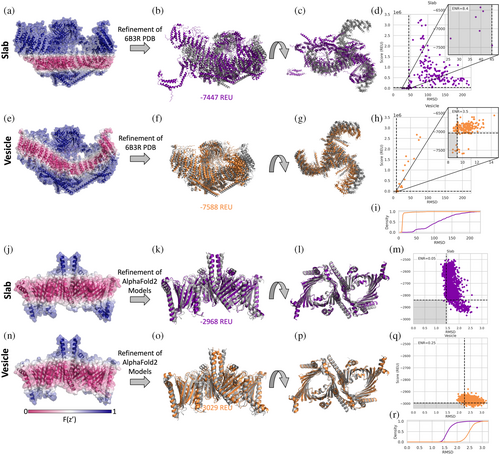
Several MPs exist in curved membranes. To take curvature into account we have implemented a vesicle geometry where the user would set the vesicle radius to define the degree of curvature. The vesicle radius is the distance from the center of the vesicle to the center of the membrane. We tested refinement in a curved membrane on the mechanosensitive channel Piezo 1 (PDB ID 6B3R). The curve of the detergent micelle around Piezo 1 can clearly be seen in the cryo-EM images (fig. 2 in Guo & MacKinnon, 2017). When the slab transition function is mapped onto the structure it is clear that it does not properly represent the hydrophobic environment needed (Figure 3a). The result of running high-resolution refinement with this poor membrane placement is evident from the large structural changes in the output models as compared to the input structure (Figure 3b–d), refinement essentially breaks up the protein. Even the lowest scoring model with the slab geometry has an RMSD of 26 Å with large changes compared to the starting structure shown in gray (Figure 3b–d). The vesicle transition function with a radius of 120 Å (based on PPM 3.0 predictions) better fits the membrane geometry in Piezo 1 (Figure 3e). The lowest scoring model is much closer to the starting structure for the vesicle geometry (~8Å, Figure 3f,g). While both geometries also produce models that have large positive scores due to clashes, the percentage of low-scoring, high-quality models is much higher for the vesicle geometry than for the slab (Figure 3d,h). Enrichment is a scoring metric measuring how many of the 10% most favorable models based on score (horizontal dotted line in Figure 3d,h) also are part of the top 10% based on RMSD (vertical dotted line in Figure 3d,h); if the top 10% of both categories overlap completely the enrichment will be 10 and if none of them are the same the enrichment is 0 (Kuenze et al., 2019). In this case, the slab model has a higher enrichment value indicating the change in scoring may not be improving the discrimination power. However, quality of models sampled is highly improved (Figure 3i) and the higher enrichment value for the slab model may be an artifact of their being so few low RMSD models similar. In another curved membrane example of potassium chloride cotransporter KCC2, the slab geometry also results in more high scoring, low-quality models (Figure S3c,f). In this case though, the slab geometry still also produces several low RMSD, low scoring models, potentially because the difference in the implicit membrane from the slab and vesicle geometries are not as great as for Piezo 1 (Figure S3a,d). ThFe enrichment values are similar in this case, but there are more lower RMSD models sampled (Figure S3g).

2.8 Refinement and scoring of AlphaFold2 models in a curved membrane

The TOM complex (translocase of the outer membrane) was recently determined by cryo-EM (PDB ID 6UCU) (Tucker & Park, 2019). PPM 3.0 predicts that TOM complexes induce membrane curvature with a radius of ~180 Å (Lomize et al., 2022). How the TOM complex structure would be scored in the slab and vesicle geometries can be seen by mapping the transition function values onto the structure (Figure 3j,n). As a demonstration of how one could use this implementation in combination with other tools, we used AlphaFold2 multimer (Richard et al., 2022) to predict the structure of the TOM complex from the sequence. Then, we used the FastRelax protocol to optimize and score the predicted models in the slab and the vesicle implicit membrane geometries. The lowest scoring models for both slab (Figure 3j,k) and vesicle geometries (Figure 3o,p) are similar to the determined structure shown in gray. While the slab geometry results in output models with slightly lower RMSD values to the PDB structure (Figure 3r), they have a much larger range of scores, indicating that the refinement cannot find an ideal fit of the flat membrane around the protein. Almost all the models from the vesicle geometry have lower scores than the models from the slab geometry (Figure 3l,p), indicating a better fit of the protein in the vesicle than in the slab model.

2.9 Modeling two membranes provides a more accurate representation of membrane protein systems spanning different bilayers

Another limitation of previous implicit membrane energy functions is only being able to account for one membrane per system. While one membrane is often sufficient, this ignores cases where one protein complex spans two membranes, such as in gram negative bacteria. Here we introduce a double vesicle option that represents the membrane as two vesicles, sharing a single origin but with different radii. One can approximate two flat membranes by setting a large radius for the vesicles, such as 1000 Å.

2.10 Implicit membrane for lipid bilayers of two interacting cells

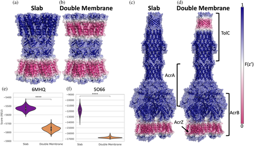
The first example we tested is a gap junction channel, where two transmembrane proteins in lipid bilayers of different cells are forming the gap junction. We used the connexin 46 gap junction channel (PDB ID 6MHQ) as a starting structure (Myers et al., 2018) and refined this structure in both the original slab membrane and in a double membrane. The value of the transition function was mapped onto the structure to visualize the membrane environment for each case (Figure 4a,b). The double membrane models all have lower scores than slab models (Figure 4e). This drop in score can be attributed to the fa_water_to_bilayer term which evaluates to zero when residues are sufficiently far from the membrane (Alford et al., 2020). Therefore, including the second membrane results in more residues with negative fa_water_to_bilayer values. The output models are similar for both geometries and the lowest scoring models overlap well with the starting structure (Figure S4a).

2.11 Implicit membranes for inner and outer membranes of gram-negative bacteria

The second example we tested was the AcrABZ-TolC efflux pump (PDB ID 5O66) (Wang et al., 2017). The transition function values for the slab (Figure 4c) and the double vesicle (Figure 4d) are mapped onto the structure to visualize the membrane for each case. In this complex, TolC is embedded in the outer membrane, while the AcrB and AcrZ subunits are embedded in the inner membrane (Figure 4d). The AcrA subunit is in the periplasm (Wang et al., 2017). Similar to the previous gap junction example, we see a drop in score with the double membrane simulations that can be partially attributed to more residues having a negative fa_water_to_bilayer scores since there is a second membrane (Figure 4f). Interestingly, the score distributions are much wider for models produced by slab geometry where there is a single membrane represented (Figures 4f and S4C). This results from sampling larger changes of the membrane position relative to the structure in the slab geometry compared to the double vesicle geometry, which anchors the complex better in the membrane. The larger range of scores is caused by the larger range of values in the fa_water_to_bilayer score term for the slab models than in the double membrane models. The output models generated by both geometries superimpose well with the starting structure and a similar tilt of TolC with respect to the rest of the complex is observed for both geometries (Figure S4B).

2.12 Incorporating experimental model membrane systems geometries in computation leads to more accurate models

For most structure determination methods, MPs must be extracted from the plasma membrane and reconstituted into a model membrane system. The composition and shape of the model membrane systems can impact the conformation of MPs. Having the ability to model MPs in geometries similar to the model membrane system in which the structure was determined in (or in which restraints were acquired) may provide additional insight into how model membrane systems introduce artifacts in MP structure and function. We use the ellipsoid model to capture the shape of model membrane systems including micelles and bicelles.

2.13 Protein–protein docking in experimentally relevant membrane geometry leads to better model discrimination

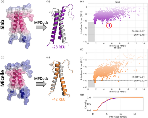
To demonstrate how modeling MPs in model membrane system geometries can be useful, we ran the protein–protein docking protocol, MPdock (Leman et al., 2015), on the glycophorin A homodimer, each with a single membrane spanning domain (Bormann et al., 1989). The structure of glycophorin A was determined by NMR in detergent micelles (MacKenzie et al., 1997). The MPdock protocol consists of two parts: a pre-optimization step where the single chains are pulled apart and optimized, and the docking step. Each step was run using either the slab or micelle geometry. The transition function values for the slab and micelle geometries are mapped on the input structure (Figure 5a,d). The lowest scoring models for each geometry are superimposed onto the starting structure (PDB ID 1AFO) shown in gray (Figure 5b,e). The output models of the final step for each geometry are evaluated using the interface score versus the interface RMSD (Figure 5c,f), indicating that the models produced with the micelle geometry result in lower scores. The score function is also better able to discriminate lower RMSD models using the micelle geometry as indicated by the funnel metric (Pnear) value of 0.63 compared to 0.06 for the slab geometry. Pnear ranges from zero to one, where higher values indicate the metrics' (in this case the interface score) ability to favor conformations with lower RMSD value (Bhardwaj et al., 2016). While models produced by the slab and micelle geometries have the same RMSD distribution (Figure 5g), the incorrect interface would be identified as the best scoring model based on the interface score with the slab geometry, circled in red in Figure 5c. The correct interface is identified based on the interface score with the micelle geometry (Figure 5f). We see a similar effect with DockQ and fraction of native contacts recovered (Fnat) where more of the lowest scoring models produced with the micelle geometry also correspond to the models with higher DockQ and Fnat scores (Figure S5) (Basu & Wallner, 2016). The ability to use score to discriminate models more like the native docking pose is important because score is one of the main metrics used to rank and choose models for docking predictions you do not already know the answer to. According to the DockQ score classification used, the slab geometry produced 0 high quality, 637 medium quality, and 910 acceptable quality models out of 2500 total models. The micelle geometry produced 1 higher quality, 667 medium quality, and 961 acceptable quality out of 2500 total models.

2.14 Refinement of transmembrane helix in membrane geometry similar to experiment results in models more similar to experimental structure

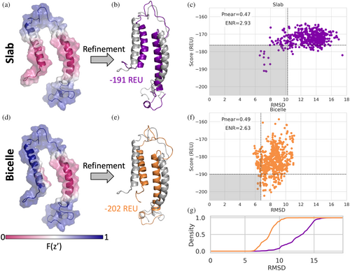
The structure of KCNE3 was determined with NMR in bicelles (Kroncke et al., 2016), showing a single span MP with an N-terminal amphipathic helix. However, when scoring the models in the NMR ensemble with the traditional slab membrane model, some conformations such as the fourth conformation in the ensemble, are scored as if the N-terminal amphipathic helix was dipping into the membrane (Figure 6a). We chose to work with the fourth conformation in the NMR ensemble to highlight how the ellipsoid geometry can be utilized to more accurately model the hydrophobic environment the protein is in. This scenario is more accurately modeled using the bicelle geometry, where the N-terminal helix is now scored as if it is resting on the edge of the bicelle (Figure 6d). In fact, when this conformation is refined and scored using the slab and bicelle geometries, the bicelle geometry results in lower scoring models and lower RMSD values relative to the starting structure (Figure 6c,f,g). The relative position of the two helices with respect to each other changes for both geometries, bringing the helices closer together, which can be seen with the lowest scoring structures (Figure 6b,e), resulting in RMSD values ~7Å.

2.15 Representing geometry of model membrane systems allows separating artifacts from model membranes vs. structure determination method

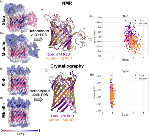
While model membrane systems can impact the protein structure, even in similar systems different structure determination techniques can result in different conformations (Koehler Leman et al., 2018). For example, the structure of outer membrane protein G (OmpG) has been determined in micelles with both NMR (DPC micelles) (Liang & Tamm, 2007) and crystallography (OG micelles) (Korkmaz-Ozkan et al., 2010). We ran refinement on the NMR model and crystal structure in both slab and micelle geometries. The aqueous environment of the pore is accounted for with both geometries, resulting in residues facing the pore having higher transition values (Figure 7a,b,e,f). The NMR model (PDB ID 2JQY) has a large loop that seemingly wraps around the micelle, but in the slab, geometry is treated like it is in the membrane (Figure 7a). In the micelle geometry with an inner radius of 8 Å this loop is scored like it is in an aqueous environment (Figure 7b). After refinement the models do not have large structural differences to the input structure (Figure 7c,d). However, the score distribution for the micelle geometry is shifted toward more negative scores as compared to the slab geometry (Figure 7d). Mapping the slab and micelle transition functions (micelle inner radius of 8 Å) onto the crystal structure (PDB ID 2X9K) does not result in large visual differences (Figure 7e,f). Refinement in both geometries sample similar structures with scores in the same range (Figure 7g,h).

5.1 Implementation of implicit membrane geometries

5.2 Applications to setup membrane geometries

We created two applications to help the user choose and visualize the appropriate geometry parameters. The mp_optimize_geometry_params application takes a PDB file, spanfile, and specified geometry as input and returns a text file with recommended parameters for the given geometry. A spanfile defines which regions of the protein are expected to span the membrane. The format of a spanfile and details on creating one can be found in the supplement. The application tries to best match the residues that are scored in a hydrophobic environment to the residues that are defined to span the membrane in the provided spanfile. The mp_transition_bfactor application helps the user visualize how their MP of interest is being scored in the implicit membrane by mapping the transition function value for each atom into the b factor column of a PDB file. The value in the b factor column can be visualized in biomolecule visualization software such as Pymol or Chimera. This application is useful for checking that the protein is positioned in the membrane and the membrane is shaped as expected before moving on to run other applications.

5.3 Choosing parameters for membrane geometries

For accurate results, the user will want to ensure they choose appropriate parameters for the membrane geometry depending on their system. The first step in choosing parameters for the membrane geometry is to decide on which geometry to model your protein in: slab, ellipsoid (micelle or bicelle), vesicle, or double membrane. Users should make this decision based on the system or the experimental setup for their use case. If the user is unsure if their MP of interest should be modeled in a curved membrane, the structure can be ran in PPM 3.0 to see if the protein is predicted to exist in a curved membrane (Lomize et al., 2022). Once deciding the geometry, the next step is creating a spanfile, which defines the residues that are expected to span the membrane. More details on a spanfile can be found in the supplement. Keep in mind, that the mp_optimize_geometry_params application is sensitive to which residues are defined in the spanfile, so it is important to have an accurate spanfile if you are planning on using that application. After creating the spanfile, the next step will depend on the chosen geometry. For a micelle or bicelle geometry, PPM 3.0 is not applicable, therefore, the user can use the mp_optimize_geometry params application to get an initial radius value. For a curved or double membrane, one can use either the PPM 3.0 or the mp_optmize_geometry_params application. The PPM 3.0 webserver was developed with the goal of estimating the expected radius of curvature and distance between two membranes, therefore, it is recommended to start with parameters from PPM 3.0 when possible. For a curved membrane, the radius of curvature provided by PPM 3.0 can be used as the vesicle radius. For a double membrane, PPM 3.0 provides a PDB file with HETATMS that represent the membranes. The distance between membranes can be calculated by determining the distance between the membranes using the position of the HETATMS (Figure S7). The mp_optimize_geometry_params application can also be used for getting initial, but keep in mind the parameters are recommended based on matching hydrophobic regions to the residues defined in the spanfile, not on physics-based energy calculations. Once the initial parameters are decided, the user should visualize the membrane determined by these parameters by using the mp_transition_bfactor application and their preferred biomolecular visualization software. It may be necessary to finetune parameters through this visualization check. Additionally, for any application using the micelle or bicelle geometry, the greatest distance between any two points within 3 Å of the XY plane at the membrane center is calculated. If the inner radius is less than half that distance, then a warning is printed out that the protein may be larger than the bicelle/micelle. For most cases, the bicelle/micelle should be larger than protein at the membrane center; however, for some structures this is not true because of soluble domains wrapping around the model membrane systems such as for KCNE3.

5.4 Protein design with pore

The protein design analysis is based on the MP Sequence Recovery benchmark test implemented within the Rosetta test server framework (Alford et al., 2021; Koehler Leman et al., 2021). Since we were specifically looking at how inclusion of the pore affected the sequence recovery, we used a subset of the original dataset of only MPs that included a pore (Koehler Leman et al., 2017). The pore functionality was turned off using the -has_pore 0 flag. To note, by including this flag with either 0, 1, or empty, the pore is not calculated. We ran the fixed-backbone design protocol three times with one designed sequence output for each case. The metrics reported in Figure 2 were calculated for each run and the average of the three independent runs is plotted. Residues were classified as pore-facing if $$$ {f}_{cavity}>0.1 $$$ and $$$ {f}_{thk}<0.75 $$$, from Equation (2).

5.5 Relax on piezo 1

We used PDB ID 6B3R for the starting structure of Piezo 1, downloaded from the OPM database. The preparation and orientation of the structure is described in detail in the supplemental protocol capture. After orientation a spanfile was generated using the mp_span_from_pdb Rosetta application. We used the mp_transition_bfactor application to visualize the implicit membrane on the structure. We ran the FastRelax protocol using the franklin2019 energy function with either the slab or vesicle geometry with a radius of 120 Å generating a total of 200 structures for each geometry.

5.6 AlphaFold2 and Rosetta relax on mitochondrial TOM complex

We used AlphaFold2 multimer (Richard et al., 2022) to generate initial decoys for the mitochondrial TOM complex. The chain sequences from PDB ID 6UCU were used as input (Tucker & Park, 2019), with five multimer predictions per model, making a total of 25 models. These models were used as input to a FastRelax protocol using the franklin2019 energy function with either the slab geometry or a vesicle geometry with a radius of 180 Å, based on reported radius of curvature from PPM 3.0 (Lomize et al., 2022). For each of the 25 AlphaFold2 predictions, 80 structures were generated by the FastRelax protocol for a total of 2000 structures for each geometry.

5.7 Relax on gap junction channel and AcrABZ-TolC multidrug efflux pump in double membrane geometry

The structure for the gap junction channel was obtained by downloading PDB ID 6MHQ (Myers et al., 2018) from the OPM webserver (Lomize et al., 2006; Lomize et al., 2012). The spanfile created using mp_span_from_pdb application corresponds to the residues that span the inner membrane. The double_vesicle_distance was set at 40 and the inner vesicle radius was set to 1000 Å. We ran FastRelax protocol using franklin2019 to produce a total of 450 structures in both the slab and double vesicle geometries.

The structure for the AcrABZ-TolC multidrug efflux pump was obtained by downloading PDB ID 5O66 (Wang et al., 2017) from the OPM webserver (Lomize et al., 2012). The double_vesicle distance was set to 244 Å and the inner vesicle radius was 1000 Å. We ran FastRelax protocol using franklin2019 to produce a total of 200 structures in both the slab and double vesicle geometries.

5.8 Docking glycophorin a in micelle geometry

To dock glycophorin A we followed the steps described in Alford, Samanta, and Gray (Alford et al., 2021) for protein–protein docking using the franklin2019. We chose to use the first conformation in the NMR ensemble for PDB ID 1AFO. We did both the prepacking and docking steps in the slab and bicelles geometries, so the geometry stayed consistent throughout the protocol. We created 50 models during the prepacking step and used the lowest scoring model as input into the docking step. We output 5000 models for the docking step. The bicelle inner radius was set at 1 Å.

5.9 Relax KCNE3 in bicelle geometry

The NMR conformational ensemble PDB ID 2NDJ (Kroncke et al., 2016) was downloaded from the PDB and from the OPM webserver. We chose to use the fourth conformation in the NMR ensemble since the amphipathic helix was positioned beside the transmembrane helix, where in the slab geometry it would be scored as if it was dipping into the membrane (Figure 6A). For both the slab and bicelles geometries 1000 output models were produced with the FastRelax protocol using franklin2019. The bicelles inner radius was set to 2 Å. The RMSD was calculated with respect to the starting structure, the 4th conformation from PDB ID 2NDJ.