Residue-level global and local ensemble-ensemble comparisons of protein domains
Abstract
Many methods of protein structure generation such as NMR-based solution structure determination and template-based modeling do not produce a single model, but an ensemble of models consistent with the available information. Current strategies for comparing ensembles lose information because they use only a single representative structure. Here, we describe the ENSEMBLATOR and its novel strategy to directly compare two ensembles containing the same atoms to identify significant global and local backbone differences between them on per-atom and per-residue levels, respectively. The ENSEMBLATOR has four components: eePREP (ee for ensemble-ensemble), which selects atoms common to all models; eeCORE, which identifies atoms belonging to a cutoff-distance dependent common core; eeGLOBAL, which globally superimposes all models using the defined core atoms and calculates for each atom the two intraensemble variations, the interensemble variation, and the closest approach of members of the two ensembles; and eeLOCAL, which performs a local overlay of each dipeptide and, using a novel measure of local backbone similarity, reports the same four variations as eeGLOBAL. The combination of eeGLOBAL and eeLOCAL analyses identifies the most significant differences between ensembles. We illustrate the ENSEMBLATOR's capabilities by showing how using it to analyze NMR ensembles and to compare NMR ensembles with crystal structures provides novel insights compared to published studies. One of these studies leads us to suggest that a “consistency check” of NMR-derived ensembles may be a useful analysis step for NMR-based structure determinations in general. The ENSEMBLATOR 1.0 is available as a first generation tool to carry out ensemble-ensemble comparisons.
Introduction
Biological macromolecules are highly dynamic entities that sample many conformations through vibrational motions, rotations around backbone and side chain torsion angles, and hinge bending motions, and may even have different low energy conformations depending on their environment. In addition, experimental and predictive modeling approaches are associated with uncertainties that vary for different parts of the model. For these reasons, an ensemble of structures is often a more accurate and complete way to represent a molecular structure than is a single discrete conformation. Although X-ray crystallographic determinations of macromolecular structures most commonly lead to a single set of coordinates representing an average structure, it has been noted that an ensemble of conformations created based on a single crystal structure analysis, or a composite of multiple crystal structures, or an ensemble of predicted or NMR derived structures may better represent a protein's native state.1-8 The variability that exists between models in an ensemble provides a wealth of information about the reliability and/or the molecular motions and variability. For instance, it has recently been shown that modeling alternate conformations marginally visible in room temperature protein crystal structures, effectively making an ensemble of models, offers insight into conformational changes related to the protein's functionality.9
With the widespread use of ensembles, especially to represent macromolecular structures determined by NMR, has come some basic protocols for their analysis. In particular, precision on a per-atom basis is routinely defined as the root-mean-square (rms) deviation of the model members from an energy-minimized “average” structure.10, 11 However, even for this purpose, the best way to overlay the ensemble members to calculate the “average” structure has not been standardized. Overlays are often performed based on all backbone or Cα atoms as well as based on a subset of such atoms from “ordered” residues subjectively defined by casual inspection of the initial overlay based on all atoms.12-15 Or one may use a program that more objectively weights atoms to optimize the superimposition. Three of these are: THESEUS, an approach that superimposes structures using all atoms with maximal likelihood derived weights16; CYRANGE, part of the CYANA software package that automatically identifies residue ranges to guide superposition14; and SuperPose, a web server that defines regions to use for superposition by comparing difference distance matrices based on α-carbons.13
As far as we are aware, although, visual inspection (as in Fig. 6 of Ref. 4) is the only common approach for directly comparing full protein ensembles with each other or with single models, as quantitative comparisons typically replace the ensemble with a representative single structure such as a minimized “average” or “medial” model,3, 17, 18 despite the loss of information this entails. Also, often only a single global comparison measure is reported such as a root mean square deviation or the global distance test score (GDT.TS) that does not provide residue or atom level details of how the models/ensembles differ,19-21 even though residue level information would be useful for discovering differences that are potentially related to molecular function or to shortcomings in experimental restraints or in the energy functions used to derive the structures.
Here, we describe a strategy to overcome these limitations by directly comparing protein structure ensembles in a way that allows rapid identification at the atom and residue level of all of the most significant global and local backbone conformational differences between them. The essential strategy, as implemented in the program the ENSEMBLATOR, is to compare the levels of intraensemble and interensemble variation and to identify the regions of greatest similarity between any members of the two ensembles. For global comparisons, the ENSEMBLATOR uses a novel approach to define a set of common core atoms by which all models are overlaid. Here, we first describe the method and then provide illustrative applications of the ENSEMBLATOR to four cases: (i) a standard precision analysis of an NMR-derived ensemble of Ribonuclease (RNase) Sa22, (ii) a comparison of that NMR ensemble with two chains from a crystal structure of RNase Sa24, (iii) a consistency analysis of the NMR-derived ensemble of RNase Sa, and (iv) comparisons to a reference crystal structure of three ensembles for a protein generated by different NMR structure refinement approaches. These examples illustrate the utility of direct ensemble-ensemble comparisons as a part of validating, refining, and analyzing ensembles.
Strategy
In this article, we use the word ensemble in referring to any set of models that are treated as one group for the purposes of a given comparison. In addition, here we use the variables m and n, respectively, to refer to the numbers of models in the first and second ensembles being compared in a given ENSEMBLATOR run [Fig. 1(A)]. If either m or n is zero that would imply that only a single ensemble is being analyzed. The essential information generated by the ENSEMBLATOR for each atom or residue are the levels of intraensemble variation for the two ensembles being compared, as well as the inter-ensemble variation and the closest approach of any member of the two ensembles [Fig. 1(A)]. These four quantities can be compared to discover regions of systematic difference. Particularly notable as the most highly significant differences between the ensembles are those regions for which the closest approach of any member of one ensemble with the other is larger than the internal variation of both individual ensembles. Additional differences, less striking but still of potential importance, are those regions for which the interensemble variation exceeds the variation of both of the individual ensembles. This strategy was developed by one of us (PAK) in the early 1990s and encoded as a set of Fortran programs (eeCORE, eeGLOBAL, and eeLOCAL); these programs are now coordinated with each other and with some Python graphing routines by the ENSEMBLATOR shell script. The ENSEMBLATOR code can be downloaded from http://biochem.science.oregonstate.edu/structural-resources/.
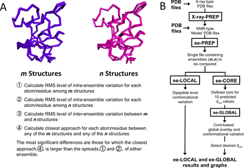
The ENSEMBLATOR strategy. A: Given two ensembles as input, one containing m structures (purple) and one containing n structures (pink), the ENSEMBLATOR strategy involves calculating the four quantities listed in points 1–4, which could be described in shorthand as spread1, spread2, spread1v2, and closest1v2. These four quantities are calculated at both the level of global conformation and the level of local backbone conformation. B: A flowchart depicting the steps and programs involved in carrying out the ENSEMBLATOR strategy for identifying regions of global and local variability.
A run of the ENSEMBLATOR requires as input a multiple-model NMR-type PDB file containing m plus n models containing exactly the same atoms in the same order. Three distinct types of runs cover the range of typical applications: first, to overlay and determine the levels of variation in a single group of structures, m would be the number of models in the group and n would be zero; second, to compare a group of structures to a single structure, m would be the number of models in the group and n would be one; and third, to compare any two groups of structures, m would be the number of models in the first group and n would be the number in the second group. In the second and third types of comparisons, the groups of structures compared may truly be sets of independently determined structures, or they may be subsets of what might in another context be considered as a single ensemble.
The steps involved in an ENSEMBLATOR run [Fig. 1(B)] begin with file preparation. If coordinates from X-ray crystal structures are to be used, the PDB file format must first be converted to that of an NMR type PDB file as can be done using the script xray.PREP. Once all the structures to be compared are in NMR type PDB files, these files are input to eePREP (ee for ensemble-ensemble), which selects the set of coordinates common to all models and writes them to a new file for the ENSEMBLATOR analyses. The global analyses are done by the pair of programs eeCORE and eeGLOBAL, with eeCORE defining a cutoff (dcut) dependent core of consistently positioned atoms and eeGLOBAL using that set of atoms to globally overlay all of the structures and produce one file containing the overlaid coordinates, a second containing a set of averaged coordinates, and a third containing the various intra and inter-ensemble global comparison statistics. The local conformation analyses are done by the program eeLOCAL, and this produces a file reporting the intraensemble and interensemble local comparison statistics. For convenience, a set of graphs are also generated that show the eeLOCAL results and that summarize the eeGLOBAL comparisons on a per residue basis for the backbone even though the raw results of eeGLOBAL are on a per atom basis and also include the side chain atoms. These plots have up to four curves and use a standard color scheme with the intraensemble variations of first and second groups being blue and green, the closest approach between any member of the two groups being red, and the intergroup variations being dashed red. In the following two sections, we describe in more detail the approaches used for the global and the local comparisons.
The global overlay approach
Carrying out global comparisons of a set of structures requires that they all be overlaid in a consistent manner. The eeCORE strategy involves selecting a core set of atoms that are positioned similarly in all m + n structures to be compared, with a user-defined cutoff value, dcut in Å, defining how close atoms must be to be considered as similarly positioned. To select this core [Fig. 2(A)], every pair of structures is subjected to a series of sequential overlays, first based on all atoms, and in each subsequent overlay based only on the subset of atoms that overlaid within dcut of each other. The process is complete when the atoms used to calculate the overlay match the atoms that have d ≤ dcut, and exactly this set of atoms is the self-consistent core for that pair of structures and that dcut. The program records for each pair the number of atoms qualifying and the root-mean-square (rms) deviation both of the core atoms and of all atoms. Tables of these numbers provide information about the structures that allows similar subgroups of the structures to be recognized [Fig. 2(B,C)]. For instance, in Figure 2(B,C) there are two natural groups of structures, one comprising structures 1 to 2 and the other comprising structures 3–6. This aspect of eeCORE was once used in a standalone manner to ascertain that a set of roughly 1000 conformations of a protein that obeyed certain distance restraints could be clustered into about 25 families of structures.25
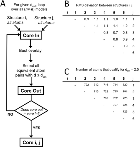
The strategy for defining a common core to use in overlay calculations. A: A flowchart of the eeCORE process used to define a self-consistent common core for a single dcut value is shown. This process is repeated for each dcut, resulting in the definition of a series of possible common cores for a user to select between. Given a set of equivalent atoms, the “best overlay” is calculated using the least-squares approach of Kabach34. B: Example output table of the rms deviations between each (i,j) pair among a group of 6 structures for a given dcut. C: Example output table of the number of atoms that were in the self-consistent core for the (i,j) pairs in panel B. Note that models 5 and 3 are the most similar having both the smallest rms deviation (0.7 Å) and the largest number of atoms (732) in their self-consistent common core.
After all pairs of structures have been compared in this way, the common core of the complete group is defined as the set of atoms that are present in every one of the pairwise self-consistent cores. We note that in this process all non-hydrogen atoms from both the backbone and side chains are used, accessing additional information compared with methods that are based only on Cα or backbone comparisons. These common core atoms are recorded in an output file (combined_coordinates_*.flag) for input to eeGLOBAL to guide the overlay on which its comparisons will be based. The eeCORE results will, of course, depend on dcut, and the most informative dcut to use will depend on the structures being analyzed and the purpose of the comparison. For this reason, the ENSEMBLATOR script has been written to automatically run through a series of 10 dcut values [Fig. 1(B)] spanning the range from a generous value that will typically allow all atoms to qualify for the common core (dcut = 50 Å) to a stringent value that will typically allow very few if any atoms to qualify in the common core (dcut = 0.5 Å). With these results in hand, users can decide which dcut to use for their primary analyses and can also carry out studies to see how robust their conclusions are to variations in dcut.
The local conformation comparison approach
The local backbone conformation of a residue in a protein is most commonly defined by its φ and ψ torsion angles, assuming, as is true for most peptide units, that the peptide adopts a trans (ω ∼ 180°) conformation. However, in comparing how similar two residues are in conformation, having two angles to compare is not ideal, as it is neither intuitive nor obvious how variations in these two angles translate into structural differences. For this reason, we developed a simple distance-based quantity that does not define individual conformations but defines how closely two conformations compare.23 We call this quantity the locally overlaid dipeptide residual (LODR), and it is calculated as follows [Fig. 3(A)]: the dipeptides are first overlaid based on the Cα, C, O, N, and Cα atoms of the peptide unit preceding the residue, and then the LODR-score is defined as the sum of the distances between the C, O, N, and Cα atoms in the subsequent peptide unit. Given this definition, no LODR values will exist for the first and last residues in a protein (as there are not complete peptide units on both sides of these residues), or for residues bordering chain breaks. The LODR distances appear to capture the structural impact of variations in φ,ψ-angles in a conceptually intuitive way, with the pattern being largely independent of the reference φ,ψ-angle and changes in φ having a much greater impact than changes in ψ [Fig. 3(B)]. The LODR distances range from 0 Å for identical conformations to ∼5 Å for conformations having their φ-values about 180° different.
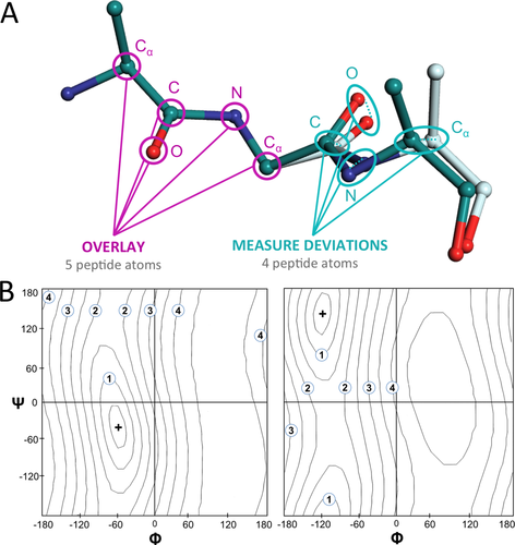
The definition of local conformational similarity used in eeLOCAL. A: The local similarity between two structures (teal and off-white carbons) is calculated for each dipeptide by first overlaying34 the Cα, N, C, and O atoms of the peptide plane preceding the residue (magenta pointers) and then defining as the LODR the sum of the distances between the C, O, N and Cα atoms in the subsequent peptide plane (turquoise pointers). B: Ramachandran plots of LODR scores for all possible conformations versus a reference residue (+) in the α-helix region (left) and β-strand region (right). Contours are at 0.5 Å intervals with integral Å contours labeled.
Results
In this section, we use test cases to explore the behavior of the novel global overlay strategy and how it compares with other available approaches, and to illustrate the utility of the ENSEMBLATOR strategy for providing useful information in the four applications listed at the end of the introduction. The test cases use two proteins: RNase Sa, a 96 amino acid enzyme having a 20-member ensemble (PDB entry 1C54) from an NMR-based solution structure determination22 and a crystal structure solved at 1.2 Å resolution (PDB entry 1RGG) with two molecules in the asymmetric unit24; and Ygdr, an uncharacterized 50 amino acid protein with an NMR-derived 20-member ensemble (PDB entry 2JN0) and a crystal structure solved at 2.7 Å resolution (PDB entry 3FIF) with eight molecules in the asymmetric unit both solved by the Northeast Structural Genomics Consortium and used in recent tests of how the Rosetta energy function can be used to improve the quality of NMR-derived structures.26
Variation in the common core size and overlay behavior as a function of dcut
Running the RNase Sa 20-member ensemble through eeCORE and eeGLOBAL with the set of 10 standard dcut values reveals the pattern of behavior we expect to see for most protein ensembles. The number of atoms in the common core decreases monotonically as dcut decreases, going from 100% of atoms at dcut = 50 Å to 0% at dcut = 0.5 Å [Fig. 4(A)]. Gratifyingly, a series of plots of the backbone rms spread of the ensemble along the chain for each dcut [Fig. 4(B)] are rather consistent for most of the dcut values. Notable variations occur at dcut below 1.5 Å for which fewer than 50% of the atoms are included in the common core. A third plot showing how the final rms backbone spread of each residue varied as a function of dcut [Fig. 4(C)] shows that the overlay of the large majority of protein atoms are moderately consistent for dcut between 2 and 4 Å, implying the choice of any of these values would yield similar results.
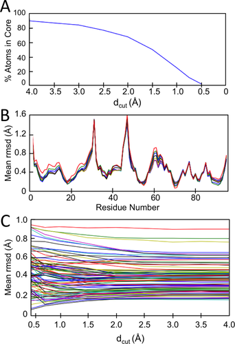
Example common core and global overlay variation as a function of dcut. A: Plotted is the percentage of atoms qualifying for the common core as a function of dcut for the 20 member RNase Sa NMR ensemble (PDB 1C54); 100% of the atoms qualify for dcut = 50 Å. B: Plots of the mean backbone rms spread around the average structure (typically used to define precision in NMR structure determinations) for each residue after overlaying the ensemble using dcut values of 50 Å (blue), 4 Å (green), 3.5 Å (red), 3 Å (cyan), 2.5 Å (magenta), 2 Å (yellow), 1.5 Å (black), 1 Å (dark blue), 0.75 Å (dark green), and 0.5 Å (red). C: A family of curves showing for each residue how the backbone rms spread around the average structure varies within dcut. Three residues with variation above 1 Å are not shown.
Comparison of global overlay quality with THESEUS, CYRANGE, and SuperPose
Using an eeCORE dcut value of 2.5 Å, we can compare the RNase Sa superposition calculated by the ENSEMBLATOR with the superpositions calculated by three other programs currently used for the same purpose: THESEUS,16 CYRANGE,14 and SuperPose.13 As seen in Figure 5(A), the qualitative patterns of variation in the ensemble along the chain yielded by the four programs are the same. Two families of curves are seen, with the statistics reported by THESEUS and CYRANGE being in a higher group and those from SuperPose being in a lower group. The eeGLOBAL output includes two measures of ensemble spread, and one of these—the rms spreads of the ensemble around the average structure—closely matches the SuperPose results, and the other—the pairwise distances between the members of the ensemble—closely matches the results of THESEUS and CYRANGE. We conclude that all four methods produce roughly equivalent results in a typical case such as this and that this provides validation for the novel eeCORE approach for defining a core to guide overlays.
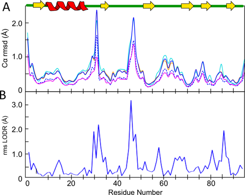
ENSEMBLATOR global and local analyses of a single NMR ensemble. A: Shown are the Cα atom rms spreads of the 20-member RNase Sa ensemble for eeGLOBAL (dcut = 2.5 Å) as measured from the average structure (blue dashed) and or between all pairs of models (blue solid). Also shown are the rms spreads output by THESEUS (cyan), CYRANGE (orange), and SuperPose (magenta). A cartoon of the RNase Sa secondary structure is shown for reference. B: Plot of the rms LODR score per residue from eeLOCAL analysis of the same RNase Sa ensemble.
Application 1: Global and local precision analysis of a single NMR ensemble
As an example of the analysis of an NMR-based ensemble, the 20 member ensemble of RNase Sa was run through the ENSEMBLATOR using m,n = 20,0 to assess the global and local precision along the chain (Fig. 5). Since there is no second group of structures to be compared, the ENSEMBLATOR output only includes the rms variations for each atom or residue of the single ensemble.
Global precision analysis
The global variation plot created using dcut = 2.5 Å [Fig. 5(A)] is nothing new, but it shows, in agreement with the analyses in the original article,22 that there are three regions of larger global variability (i.e., poorer precision) in the NMR ensemble: the N-terminus, residues 25–33, and residues 44–50. All three regions reside in loops and have variation in the 1–2 Å range.
Local precision analysis
The plot provided by eeLOCAL [Fig. 5(B)] reports the LODR score for each residue (except the first and last) and provides additional information compared with the conventional global analysis. This plot shows much sharper variability and reveals exactly which residues have conformational variation that give rise to the global variation. For instance, the variability observed in the eeGLOBAL analysis of regions 25–33 and 44–50 can be attributed largely to local variation at residues 30, 32, and 45–47. From a practical perspective, eeLOCAL identifies these residues as places where additional restraints could be sought in order to improve the precision of the structure. Conversely, while residues 39–42 and 60–62 are identified as regions of medium global variation, the eeLOCAL analysis reveals that these residues are actually quite precisely defined in terms of their local conformation.
Application 2: Comparison of an NMR ensemble with a crystal structure or crystal structure ensemble
It is common to compare solution structures to crystal structures, and in the original RNase Sa NMR structure determination, the NMR-derived ensemble was compared separately to chains A and B of a crystal structure of the same protein (see Fig. 7 of Ref. 22). Only small differences for the strands and helices were noted, and larger differences occurring in loops near residues 32, 46, and 63 and in side chains near residue 76, were explained as being due to the influences of crystal packing or, in the case of the 60s loop, to phosphate binding or salt concentration. The authors concluded that “no significant differences were detected.”
Using the ENSEMBLATOR to compare the NMR ensemble separately with chain A or chain B (using runs with m,n = 20,1), and also with a two member crystal structure ensemble consisting of both chains A and B (using a run with m,n = 20,2) provides a different picture. In the global comparisons with chains A or B [Fig. 6(A,B)], the most robustly defined differences are where the closest approach of any NMR model to the crystal structure (red solid line) exceeds the intraensemble variations of the NMR models (blue line). As seen in these plots, such differences occur for both chains A and B near residues 5, 17–21, 38–42, and 76–82; these include residues in secondary structural elements and none of them were commented on in the original report.22 The two differences originally noted in loops near residues 32 and 46 are less robustly defined because of their higher variability in the NMR structure; the difference originally noted in the 60s loop appears significant in the comparison with chain A, but not in the comparison with chain B. This variation between chains A and B emphasizes the potential value of being able to compare with both crystal structures at the same time. Such an ensemble-ensemble comparison [Fig. 6(C)] includes a fourth curve representing the intragroup variation of the X-ray models (green) and identifies residues 61–63 as a point of major variation between the X-ray structures. In this way, the ensemble-ensemble comparison effectively deemphasizes the differences with the NMR structures in the 61–63 region while reinforcing the reality and consistency of the backbone differences near residues 5, 17–21, 38–42, and 76–82.
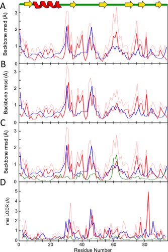
Comparison of the RNase Sa NMR ensemble with an RNase Sa crystal structure. ENSEMBLATOR (dcut = 2.5 Å) plots show the intraensemble variation in the NMR ensemble (blue), the intraensemble variation in the X-ray ensemble (green; present only when more than one X-ray model is used), the interensemble variation (red-dotted), and the closest approach between the two ensembles (red). A: eeGLOBAL comparison of the NMR ensemble to only chain A of the X-ray structure (PDB 1RGG). B: eeGLOBAL comparison of the NMR ensemble to only chain B of the X-ray structure. C: eeGLOBAL comparison of the NMR ensemble to both chains of the X-ray ensemble. D: eeLOCAL comparison of the NMR ensemble to both chains of the X-ray ensemble. A cartoon of RNase Sa secondary structure is included.
Furthermore, the eeLOCAL output for comparing the NMR ensemble with the two chain X-ray ensemble [Fig. 6(D)] identifies many residues for which the difference in local backbone conformation between the closest models (red solid curve) substantially exceeds the intraensemble variations (blue and green curves); these include residues 4, 12, 23, 38, 43, 55–7, 61–3, 75, 78, 82–3 and 89–91. Especially striking is residue 83 for which the LODR score is near the maximal possible value of 5 Å, even though the global comparison [Fig. 6(C)] does not show much discrepancy. A closer examination of this segment (Fig. 7) reveals that between the crystal and solution structures the Cα-path is similar, but the 82–83 peptide is flipped making the ψ-value for residue 82 and the φ-value for residue 83 nearly 180° different. A search using the Protein Geometry Database (PGD27) of diverse crystal structures solved at 1.8 Å resolution or better found 4011 and 38 examples of peptides having φ,ψ-angles within ±30° of those seen for residues 82 and 83 in the crystal and the NMR-based structures, respectively. In this light, both conformations are plausible, but the conformation modeled in the NMR structure is so much rarer that it would be deserving of scrutiny.
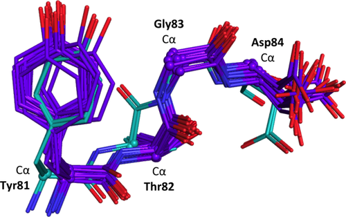
Differing peptide flip between residues 82 and 83 of the RNase Sa NMR and X-ray ensembles. Shown is a four-residue segment from the eeGLOBAL (dcut = 2.5 Å) overlay of the RNase Sa 20-member NMR ensemble (violet carbons) and from the two-chain RNase Sa X-ray ensemble (cyan carbons). The Cα atoms for each residue are shown as spheres and identified with a nearby label.
Although investigating the origins of these differences (i.e., deciphering which are real and which are a result of data or modeling limitations), such as by carrying out a joint X-ray/NMR refinement,28 is beyond the scope of this report, the example illustrates the utility of ensemble-ensemble comparisons in deriving powerfully informative residue-level information about areas of global and local difference, and also highlights how worthwhile it is to have an effective way to account for the variability that exists among crystal structures of a given protein.
Application 3: Assessing the self-consistency of an NMR ensemble
A further analysis of the RNase Sa solution structure ensemble that illustrates the utility of ENSEMBLATOR comparisons is to assess the extent to which the 20 models deposited in the PDB provide a robust sampling of the relevant conformational space.1 Because the individual models of such ensembles are supposed to be of similar quality in terms of their levels of agreement with the NMR data and their energetics, any half of an ensemble should sample a similar range of conformational space as the other half. To test how well this holds true for the RNase Sa ensemble, we compared the first 10 models in the ensemble to the last 10 (i.e., using m,n = 10,10). For the global [Fig. 8(A)] comparison, the closest approach curve (red solid) is lower than all other curves, showing that the two halves of the ensemble have no consistent systematic differences. Also, the variation among the first and second 10 models is similar, except near residue 30 where the second 10 models (green) show about five-fold the variation of the first 10 (blue).
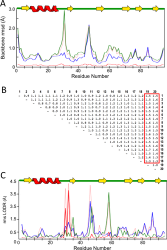
Self-consistency analysis of the RNase Sa NMR ensemble. A: eeGLOBAL (dcut = 2.5 Å) plots of the RNase Sa 20-member NMR ensemble show the intraensemble variation for the first 10 models (blue), the last 10 models (green), the variation between the two groups (red-dotted) and the closest approach between the two groups (red). B: The table of pairwise rms deviations (in Å) from the eeCORE analyses with red box highlighting differences of models 19 and 20 from the other 18 models. C: eeLOCAL comparison of the first 18 models to the last two models identifies residues 31 and 33 as having their closest similarity (red solid trace) much higher than the internal variations (blue and green traces).
To localize the structures causing the difference, we examined the tabular eeCORE output of the rms deviations for each pair of models [Fig. 8(B)], and these showed that models 19 and 20 are similar to each other and differ from the first 18 models. We then ran the ENSEMBLATOR again to compare models 1–18 with 19–20 (i.e., using m,n = 18,2). The eeLOCAL output of this comparison [Fig. 8(C)] showed distinct differences at Tyr30 and Gln32 with these residues having LODR values of 2.5–3.5 Å for the most similar conformations in the two groups (red curve) compared with internal variations near or below 1.0 Å (blue and green curves).
Looking at the structures [Fig. 9(A)] and a ϕ,ψ-plot [Fig. 9(B)] confirms that residues 30–32 adopt a different conformation in models 19–20 compared with 1–18, and that the conformation seen in models 1–18 are more similar to the conformation in the crystal structures. The ϕ,ψ-plot further shows that residues 31 and 33 in models 19–20 adopt uncommon outlier conformations.29 As above, using the PGD27 to survey diverse proteins solved at 1.8 Å resolution or better, a we found 96, 0, and 1176 segments with ϕ, ψ values within ±30° of the conformations seen in models 1–18, models 19–20, and the crystal structures, respectively. Based on this, we suggest that the conformation of this region of models 19 and 20 is not plausible. Also, given that models are typically ranked by their relative energies so that models 19 and 20 are, we presume, the highest energy models in this ensemble, we further suggest that such self-consistency checks of NMR-derived (and other) ensembles combined with PGD searches could be useful during ensemble preparation to decide at what point higher energy structures in the ensemble are not truly of comparable quality to the rest of the structures and should be deemed unacceptable.
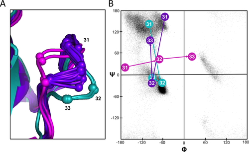
RNase Sa residues 31–33 backbone conformation in the crystal structure and the NMR ensemble. A: Shown are backbone paths for residues 31–33 of an eeGLOBAL overlay (dcut = 2.5 Å) of the RNase X-ray structure (magenta), models 1–18 of the NMR ensemble (purple), and models 19–20 of the NMR ensemble (turquoise) with the Cα atoms represented as spheres. B: Backbone torsion angles for residues 30–32 representative of each of the three groups shown on a Ramachandran plot (colors as in panel A). For reference, the background black dots show commonly populated regions as seen in crystal structures determined at 1.2 Å resolution or better.
Application 4: Comparing NMR ensembles derived by different protocols
The ENSEMBLATOR can also be used to gain insight into how different structure determination protocols can impact structure quality/accuracy. Rosetta refinement has been shown in specific cases improve NMR structure quality (e.g. Ref. 30), and recently Mao et al.26 tested 40 NMR and crystal structure pairs to see how much refinement with a standard Rosetta protocol alone or in conjunction with NMR-based restraints could increase the similarity of the ensembles with crystal structures. The level of agreement of an NMR ensemble with its corresponding crystal structure was measured only by a single overall value: the GDT.TS (Ref. 31). Here, we use the ENSEMBLATOR to reanalyze the models of Ygdr, for which restrained Rosetta refinement increased the GDT.TS from 0.77 to 0.81, a small numerical increase that provides no information about how the refinement impacted the model. As for the analyses above, we used dcut = 2.5 Å for global comparisons.
The global comparison of the original NMR ensemble with a crystal structure-based ensemble [Fig. 10(A)] shows that other than the N- and C-termini, there are four broad regions of variability within the original NMR ensemble (blue curve) at residues 7–9, 15–17, 22–24, and 32–35, and that residues 15–18 is the segment matching worst with the crystal structure. The eeLOCAL output (not shown) highlights Lys17 as having particularly poor agreement with respect to the crystal structure. After Rosetta refinement without NMR restraints [Fig. 10(B)], the internal variations near residues 17, 23, and 34 increase and the spread near residue 8 decreases dramatically, while remarkably in all four places the closest agreement of any of the NMR models with a crystal structure model improves somewhat. This implies that the Rosetta energy function is improving the sampling of conformations close to those adopted in the crystal structure. As one example, the eeLOCAL results show that at Lys17 the closest models decrease from LODR = 3.0 Å to 2.2 Å (not shown).
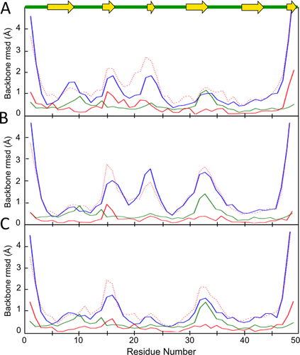
eeGLOBAL analyses provides insights into how Rosetta refinement impacts an NMR-derived ensemble. A: Shown is an eeGLOBAL plot (dcut = 2.5 Å) of the unrefined, original NMR ensemble (PDB code 2JN0; 20 models) compared with the crystal structure (ensemble based on 8 noncrystallographic symmetry related chains in PDB code 3FIF). B: Same as (A), but using the NMR ensemble after it had been refined with Rosetta. C: Same as (A), but using the NMR ensemble after it had been refined with Rosetta in the presence of the NMR restraints. The Rosetta refined ensembles used for the analyses in panels B and C were obtained from the URL: http://psvs-1_4-dev.nesg.org/results/rosetta_MR/rosettaMR_PSVS_summary.html.
Combining the NMR restraints with the Rosetta refinement [Fig. 10(C)] results in broad decreases in ensemble spread, especially at residues 22–24, indicating the synergistically distinct information content of the Rosetta energy function and the NMR-based restraints. Interestingly, at the loop near residue 33 where the crystal structure ensemble shows the greatest variation, the use of Rosetta actually makes the model slightly less similar to the crystal structures. In contrast, the two regions where Rosetta most dramatically decreased the ensemble spread and increased its agreement with the crystal structures are both β-strands (7–9, 22–24). We conclude that this type of analysis, made easy by the ENSEMBLATOR, provides much more information than does the single overall GDT.TS score reported by Mao et al.20 and such insights about how the Rosetta energy function does and does not improve models could help guide improvements in energy functions as well as structure determination protocols.
Discussion
As illustrated by the four example applications presented above, the ENSEMBLATOR approach to structural comparisons provides a useful tool that is notably more informative than current approaches used for identifying systematic differences between an ensemble and a single structure or another ensemble. In addition to the above examples, we note that a recently published study by Nyarko et al.32 used the ENSEMBLATOR to analyze the NMR ensembles of natural active and inactive variants of a fungal toxin of wheat that differ by a few point mutations. Those analyses identified a region of subtle difference that had notably higher rms spreads in the inactive form, and the authors hypothesized that the additional flexibility in this loop region was in part responsible for the inactivity.
The two most novel concepts of the ENSEMBLATOR analyses are the calculation of a “closest-approach-between-any-members-of-the-ensemble” statistic and the eeLOCAL analyses that use the LODR score to provide a convenient single distance-based measure of local backbone conformational similarity. The former innovation enhances the sensitivity with which the most significant differences can be identified in both the global and local comparisons, and the eeLOCAL analyses help pinpoint the local variations that underlie global differences. A third novel aspect of the ENSEMBLATOR is the eeCORE approach of carrying out all pairwise comparisons to identify a common self-consistent core, as well as to provide statistics that can allow subgroups of similar structures to be identified among the compared models (e.g., Ref. 24) [Fig. 8(B)]. The choice to have the ENSEMBLATOR run eeCORE for a series of dcut values for every comparison (rather than picking 2.5 Å as a generally useful standard value) provides a purposeful reinforcement of the oft-neglected reality that any given “best overlay” is just one of many that could be chosen, and as noted above, allows users to easily assess how robust their results are to the choice of the overlay parameters.
One aspect of our work with immediate implications is our unexpected finding that the last two models of the RNase Sa NMR ensemble have a segment that adopts implausible ϕ,ψ-angles. We see no reason to suspect that this is a problem unique to this particular ensemble, and suggest that doing such consistency checks during NMR ensemble generation would be a useful general application of the ENSEMBLATOR. As far as we are aware, no standard protocols exist for deciding on the most appropriate size or constitution of an ensemble, or for instance, how large an energy gap between the lowest and highest energy model is acceptable. In this light, we further suggest that it would be useful to record the relative energies of the individual models in an ensemble as part of PDB depositions.
An additional application of such ensemble comparisons would be a more facile finding of differences between modeled and experimental protein ensembles (e.g., Ref. 4), and potentially guiding the improvement of forcefields associated with modeling programs. It was, for instance, recently shown that identifying details of protein structure that were consistently predicted incorrectly very effectively guided the making of specific improvements in the Rosetta forcefield.33 Similarly specific guidance could be obtained by using eeLOCAL to compare ensembles of template-based models against crystal structures (or even better crystal structure ensembles) to locate specific systematic backbone differences that could reflect inadequacies in the force field.
We note that the limitation of the current version of the ENSEMBLATOR to have all input models with the same exact set of atoms is not a limitation in principle but could be overcome by a more sophisticated front end that could assign equivalent atoms between nonidentical structures. In concept, creating an ENSEMBLATOR version that can handle nonidentical proteins may as straightforward as using an existing program like SuperPose13 as a front end to define equivalent atoms and overlay the structures, and then feed those files to modified versions of eeGLOBAL and eeLOCAL. The other limitation worth explicitly noting is that because the eeCORE and eeGLOBAL comparisons use a single overlay, protein domains that move relative to one another should be analyzed separately, as is true for other current ensemble analysis approaches. This limitation, however, does not apply to the eeLOCAL analyses, and in fact, eeLOCAL analyses can be useful for locating specific “hinge” residues that are involved in conformational changes.
Acknowledgment
The authors thank Blaine Roberts and Donnie Berkholz for contributions to the source code.


