Data-driven finite element computation of microstructured materials
Abstract
This paper presents a model-free data-driven strategy for linear and non-linear finite element computations of open-cell foam. Employing sets of material data, the data-driven problem is formulated as the minimization of a distance function subjected to the physical constraints from the kinematics and the balance laws of the mechanical problem.
The material data sets of the foam are deduced here from representative microscopic material volumes. These volume elements capture the stochastic characteristics of the open-cell microstructure and the properties of the polyurethane material. Their computation provides the required stress-strain data used in the macroscopic finite element computations without postulating a specific constitutive model. The paper shows how to derive suitable material data sets for the different cases of (non-)linear and (an-)isotropic material behavior efficiently. The numerical example of a rubber sealing illustrates possible areas of application, and the proposed strategy's versatility.
1 INTRODUCTION
In the data-driven finite element analysis, which was recently introduced by Kirchdoerfer and Ortiz [1], the constitutive material modeling is eluded and instead, data are directly employed as an input for computational analysis. This model-free description allows to implement arbitrary constitutive relations. It can be especially beneficial when adaptions of the microstructural material design are wanted because it avoids starting a new fitting process every time such a change is made. The numerical approach was supplemented by mathematical investigations in Conti et al. [2], demonstrating that the data-driven computational mechanics comprises the classical definition of solid mechanics boundary value problems. While the original work [1] was proposed in the framework of linear elasticity, extensions to elastodynamics, non-linear elasticity and related problems followed soon, cf. [3-7].
This contribution focuses on the question of how we can use the data-driven finite element analysis for non-linear materials. Since experimental data acquisition can be tedious, we suggest using numerical computations of representative volumes. In that way, the micromechanical behavior of the material can be evaluated and homogenized data points can be deduced. Specifically, we consider polyurethane foam. Depending on the manufacturing process and the composition of the constituents, the material properties such as density, pore distribution, and structure of the material vary. To avoid fitting a material model for every case, we use stochastic representative volume elements (RVEs) to generate the data basis. A foam generator produces the RVEs with the desired properties which are then subjected to some test loads to deduce the homogenized data. To not simulate each point individually, like typically done in FE2 computations, the database is here constructed with the help of material properties such as linearity or isotropy.
In this paper, we outline in Section 2 the concept of the data-driven finite element method (DD-FEM) for finite deformation strain and stress measures and discuss the different approaches' numerical properties. We then introduce open-cell foam volumes whose microstructure is generated stochastically. In Section 3, we discuss strategies to generate the data set  for different cases of linear or non-linear and isotropic or anisotropic material behavior. Finally, we present in Section 4 the computation of a rubber sealing and close with a short summary in Section 5.
2 GOVERNING EQUATIONS
 is completely described by the deformation gradient
 (1)
(1) . The stresses fulfill the linear and the angular momentum balances
 (2)
(2) (3)
(3) . The solid is subjected to geometrical and static boundary conditions at its boundaries Γ0 and Γ1 with outward unit normal N,
 (4)
(4) (5)
(5) and
and  . These physical equations determine the set
  of mechanical admissible strain-stress states. The goal of the data-driven problem is to find the minimal distance between this constraint set and a material data set
  . The set
  consists always of tuples of a strain measure and a stress measure, for example the linear-elastic strain and stress
  , the deformation gradient together with the first Piola-Kirchhoff stress (F, P), or the right Cauchy-Green tensor with the second Piola-Kirchhoff stress (C, S).
2.1 Data-driven problem
 and its convex conjugate
  , a distance function of the form
 (6)
(6) . The corresponding data set
  contains tuples of the deformation gradient and the first Piola-Kirchhoff stress tensor. We presume them to be physical meaningful and, specifically, to fulfil Equation (3).
This results in a functional which states a non-linear data-driven boundary value problem. The unknown fields are coupled and contrained. Because the formulation cannot be solved explicitly, this problem cannot be treated with a standard finite element approach. One way to simplify it is to not enforce the angular momentum, presuming a negligible distance between the data of solution  and the material data
  in that respect. With this assumption the problem is linearized and, after discretization, we obtain the same set of finite element equations like in linear elasticity; for a derivation we refer to our work [8].
 and the corresponding second Piola-Kirchhoff stress tensor
  . To define the distance (6) we use the convex functions
 (7)
(7) (8)
(8) . After some algebraic manipulation, cf. [9], we obtain the functional to be optimized in terms of u, S, λ. A variation with respect to the displacement field,
  , gives after some re-arrangement,
 (9)
(9) , gives
 (10)
(10) , we derive the expression for the stresses,
 (11)
(11) (12)
(12)2.2 Finite element formulation
 and employ the usual ansatz for the unknown fields and their variations
 (15)
(15) contains the shape functions
  for every degree of freedom
  . The vectors
  and
and  denote the nodal displacements and Langrange parameters. The gradients are summarized in matrix
  ; the subscript e refers to one element. The finite element discretization of the system (13-14) is performed with the ansatz (15) and the deformation gradient is calculated in each integration point as
  , where
  has the suitable vector form. The discretized system of residual equations is then:
 (16)
(16)3 RECORDING OF THE MATERIAL DATA SETS
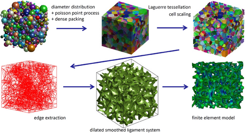
The material data sets required for the DD-FEM are gained from systematic computations of microscopic RVEs. Exemplarily we consider open-cell polyurethane foam, which is a rubbery material with a relative density of less than  . The foam's mechanical behavior is determined by the polyurethane matrix material and the cellular microstructure, consisting of a network of ligaments connected at junctions. An accurate description relies on the natural foam's geometry, whose topological characteristics are gained from computed tomography scans for example. Assuming these characteristics, for example the pore volume fraction, the size distribution, the coefficient of variation, and the anisotropy factor, to be known, the generation of the stochastic foam element follows the procedure outlined in Figure 1 and described in detail in the literature [10].

 are treated equally and denoted as
  subsequently.
 of the RVE is prescribed and the stress field is computed with a linear or non-linear FEM. The homogenized stresses
  are derived by

 and
and  provides one data tuple. The data sets, which are used as an input for the DD-FEM, are the collections of all
  tuples or, with
  all
all  tuples. Since only one data point is determined per RVE simulation and these can be very expensive, the question arises as to how many points are required for a DD-FEM calculation. Our experience suggests a minimum number of
  data tuples per stress component, which results in the computation of n6 tuples for three dimensions. That many simulations can not be deduced for detailed and representative microscopic structures. Therefore, we will discuss in the following how it is possible to speed up the whole process of DD-FEM calculations with RVE data.
Case A: non-linear and anisotropic material
For the general situation of a direction dependent and non-linear material response, for example a viscoelastic foam with elongated pores in one direction, simplifications are difficult. Here only a brute force approach of one RVE computation for every  or
or  tuple gives the desired data set
  . Such a strategy corresponds to a FE2 computation and is hardly feasible with our detailed stochastic RVEs.
Case B: non-linear and isotropic material
 ,
,  d, and then transform the resulting principal stresses,

 . For n6 data then n3 computations are needed.
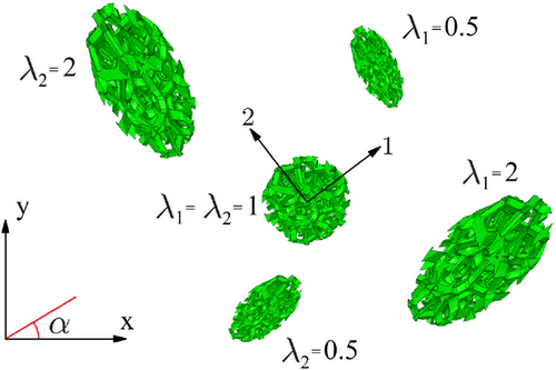
Case C: linear and anisotropic material

 . Conveniently, unit loads as displayed in Figure 3 are computed and evaluated. This strategy leads to a enormous decrease of computational effort.
Case D: linear and isotropic material
In the simplest case of isotropic, linear (elastic) material the loading scenarios simplify even more. The material's isotropy makes it possible to describe the material by only two states, namely one of the three elongations and one of the three shear states from Figure 3. All other data tuples can be gained by linear combinations and rotations of the coordinate system.
Note that for all simplifications the RVEs are assumed to give the same averaged response, that is, we neglect here the noise induced by the stochastic generation.
4 NUMERICAL EXAMPLE
As a computational example we present a plane-strain computation of a sealing made of a foamy rubber material. The rubber is a Neo-Hookean material, extended to the compressible range, with  , and parameters of polyurethane,
  MPa and
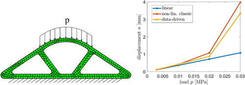
  MPa−1. The mesh of the sealing, its loading and boundary conditions are shown on left-hand side of Figure 4. The component is fixed in the vertical direction. For the distributed surface load p four different values are used, namely
  kPa,
kPa,  kPa,
kPa,  kPa and
  kPa. A linear (material and kinematic) and a non-linear (material and kinematic) finite element analyses with homogenized material data are used for comparison. More details as well as a three-dimensional analysis of the sealing can be found in the literature [9].
The 2D-RVE used for data generation is a simple 7 × 7 mm2 square with four regularly arranged pores of radius 2 mm meshed with 2601 finite elements which was fast and easy to compute in the commercial program Abaqus. The 2D-RVE is isotropic but because of the non-linear material it corresponds to Case B of Section 3. The principal stretches λ1 and λ2 are varied in 51 steps between 0.8…1.2 which lead to 2601 non-linear finite element computations. The resulting data set has  data tuples that provide the initial set
  of our data-driven computation.
To reduce these computational costs of the DD-FEM, we apply the multi-level method introduced in the literature [11]. In this procedure we compute the solution on smaller (coarser) subsets,  . After a computation at level l with data set
  , relevant data are added to the next set
  . Here, the data-driven computations were run on three levels of refined data sets.
On the right-hand side of Figure 4 the computed load-displacement curves are shown for the data-driven solution and two standard FEM computations. Recorded is the displacement of the center top nodes, where we have the largest displacement. It can be seen that the data-driven solution, computed with the non-linear material data but the linearized kinematic formulation of Section 2.1, gives a somewhat stiffer response than a fully non-linear Neo-Hookean model. The difference in the maximal displacement is about 15% for moderate straining. We remark that a fully non-linear kinematic of the DD-FEM comes at the price of a much higher computational effort. In that respect, the linearized data-driven response describes the deformation of the structure sufficiently.
In Figure 5 the horizontal Cauchy stress component  is displayed for
  kPa. A good agreement of the standard FEM solution and the data-driven solution of level 2 has been reached.
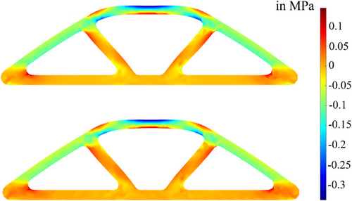
 for a linear FEM solution (top) and the DD-FEM solution (bottom) at a surface load of
  kPa. DD-FEM, data-driven finite element method.
5 CONCLUSION
In this paper, we propose a strategy to provide the necessary material database for linear and non-linear data-driven finite element computations. Typically, such data are presumed to be available from experimental investigations but here we suggest a computational material testing instead. With representative material volumes the micro-scale problem is investigated and the derived homogenized data give the input for the solution of the macro-scale problem.
Specifically, we consider data-driven computations of components made of open-cell foam. The RVEs map the foam's characteristics, such as pore volume, distribution, and pore and ligament geometry. In conjunction with simplifications made possible by the spatial material behavior, the computation enables us to generate the material data input set efficiently.
ACKNOWLEDGMENTS
We gratefully acknowledge the support of the DFG as part of the Priority Program SPP1886 “Polymorphic uncertainty modelling for the numerical design of structures” under the grant WE2525/10-1 and WE2525/10-2.
Open access funding enabled and organized by Projekt DEAL.


 for the sake of clarity,


