Understanding recent deep-learning techniques for identifying collective variables of molecular dynamics

1 INTRODUCTION

Molecular dynamics (MD) simulation is a mature computational technique for the study of biomolecular systems. It has proven valuable in a wide range of applications, for example, understanding functional mechanisms of proteins and discovering new drugs [1, 2]. However, the capability of direct (all-atom) MD simulations is often limited, due to the disparity between the tiny step-sizes that the simulations have to adopt in order to ensure numerical stability and the large timescales on which the functionally relevant conformational changes of biomolecules, such as protein folding, typically occur.

One general approach to overcome the aforementioned challenge in MD simulations is by utilising the fact that in many cases the dynamics of a high-dimensional metastable molecular system can be characterised by a few features, that is, collective variables (CVs) of the system. In deed, many enhanced sampling methods (see ref. [3] for a review) and approaches for building surrogate models [4-7] rely on knowing CVs of the underlying molecular system. While empirical approaches and physical/chemical intuition are still widely adopted in choosing CVs (e.g., mass centres, bonds, or angles), it is often difficult or even impossible to intuit biomolecular systems in real-life applications due to their high dimensionality, as well as structural and dynamical complexities.

Thanks to the availability of numerous molecular data being generated and the rapid advance of machine learning techniques, data-driven automatic identification of CVs has attracted considerable research interests. Numerous machine learning-based techniques for CV identification have emerged, such as the well-known principal component analysis (PCA) [8], diffusion maps [9], isometric feature mapping (ISOMAP) [10], sketch-map [11], time-lagged independent component analysis (TICA) [12], as well the kernel-PCA [13] and kernel-TICA [14] using kernel techniques. See refs. [15, 16] for reviews. The recent developments mostly employ deep learning techniques and largely fall into two categories. Methods in the first category are based on the operator approach for the study of stochastic dynamical systems. These include variational approach for Markov processes using neural networks (VAMPnets) [17] and the variant state-free reversible VAMPnets (SRV) [18], the deep-TICA approach [19], and Invariant subspaces of Koopman operators learned by a neural network (ISOKANN) [20], which are capable of learning eigenfunctions of Koopman/transfer operators. The authors of this paper have also developed a deep learning-based method for learning eigenfunctions of infinitesimal generator associated to overdamped Langevin dynamics [21]. Methods in the second category combine deep learning with dimension reduction techniques, typically by training autoencoders [22]. For instance, several approaches are proposed to iteratively train autoencoders and improve training data by “on-the-fly” enhanced sampling. These include the Molecular Enhanced Sampling with Autoencoders (MESA) [23], Free Energy Biasing and Iterative Learning with Autoencoders (FEBILAE) [24], the method based on the predictive information bottleneck framework [25], the Spectral Gap Optimisation of Order Parameters (SGOOP) [26], the deep Linear Discriminant Analysis (deep-LDA) [27]. Besides, various generalised autoencoders are proposed, such as the extended autoencoder (EAE) model [28], the time-lagged (variational) autoencoder [29, 30], Gaussian mixture variational autoencoder [31], and EncoderMap [32].

Motivated by these rapid advances, in this paper we study the aforementioned two categories of deep learning-based approaches for finding CVs, that is, approaches for computing leading eigenfunctions of transfer operator associated to the underlying dynamics and approaches that learn an autoencoder via minimisation of reconstruction error. The remainder of this article is organised as follows. In Section 2, we present the approach for CV identification based on computing eigenfunctions of transfer operator. We present a variational characterisation, as well as a loss function for learning the eigenfunction. In Section 3, we study autoencoders. In particular, we present a characterisation of the optimal (time-lagged) autoencoder. In Section 4, we illustrate the numerical approaches for learning eigenfunctions and autoencoder by applying them to two simple yet illustrative systems.

2 EIGENFUNCTIONS AS CVs FOR THE STUDY OF MOLECULAR KINETICS ON LARGE TIMESCALES

In this section, we consider eigenfunctions of transfer operator associated to the underlying dynamics. Approaches for computing eigenfunctions of infinitesimal generator and further motivations of eigenfunctions can be found in the extended version of this paper [33].

Transfer operator

Transfer operator approach offers an effective way to study dynamical systems without specifying the governing equations [34, 35] and is hence widely adopted in developing numerical algorithms. In this framework, one assumes that the trajectory data is sampled from an underlying (equilibrium) system whose state y at time given its state x at time t can be modelled as a discrete-time Markovian process with transition density , for all , where is called the lag-time and the process is assumed to be ergodic with respect to the unique invariant distribution μ, defined by

(1)

where Z is a normalising constant. The transfer operator associated to this discrete-time Markovian process is defined as [35]

(2)

for a density (with respect to μ) . Assume that the detailed balance condition is satisfied, that is, for all . Then, we can derive

(3)

which shows that in the reversible setting the transfer operator coincides with the semigroup operator (at time τ) associated to the underlying process [36]. One can show that is self-adjoint in with respect to the inner product . Also, for a function we define the energy

(4)

which is related to the transfer operator by the identities , where is the identity map (see ref. [33, Lemma 1]). In particular, one can conclude that all eigenvalues of are no larger than one. We assume that the spectrum of consists of discrete eigenvalues

(5)

and the largest eigenvalue (corresponding to the trivial eigenfunction ) is non-degenerate. These eigenvalues and their corresponding eigenfunctions are of great interests in applications, since they encode information about the timescales and metastable conformations of the underlying dynamics, respectively [34, 35].

Variational characterisation and loss function

In the following, we record a variational characterisation of eigenfunctions of transfer operator. Such characterisation is useful in developing numerical algorithms [37, 38], in particular in designing loss functions in recent deep learning-based approaches [17, 18, 21]. In fact, using the same proof of ref. [21, Theorem 1], we can show the following variational characterisation for eigenfunctions of transfer operator.

Theorem 2.1.Let and . Assume that has discrete spectrum consisting of the eigenvalues in (5) with the corresponding eigenfunctions , . Define . We have

(6)

where is the energy defined in (4), and the minimisation is over all under the constraints

(7)

Moreover, the minimum in (6) is achieved when for .

Theorem 2.1 motivates the following loss function for learning eigenfunctions of the transfer operator :

(8)

where α is a penalty constant, denotes the empirical mean with respect to the joint distribution 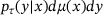, and Var^data, Cov^data denote empirical estimators of the variance and co-variance with respect to the measure μ, respectively. For brevity, we omit further discussions on the loss (8), and we refer to refs. [21, Section 3] and [33] for more details.

Compared to VAMPnets [17], the loss (8) imposes orthogonality constraints (7) explicitly and directly targets the leading eigenfunctions rather than basis of eigenspaces. Also, as opposed to the approach in ref. [18], training with the loss (8) does not require backpropagation on matrix eigenvalue problems.

3 ENCODER AS CVs FOR LOW-DIMENSIONAL REPRESENTATION OF MOLECULAR CONFIGURATIONS

In this section, we briefly discuss autoencoders in the context of CV identification for MD.

An autoencoder [22] on is a function f that maps an input data to an output by passing through an intermediate (latent) space , where . It can be written in the form , where and are called an encoder and a decoder, respectively. The integer k is called the encoded dimension (resp. bottleneck dimension). In other words, under the mapping of the autoencoder f, the input x is first mapped to a state z in the latent space by the encoder , which is then mapped to y in the original space by the decoder . In practice, both the encoder and the decoder are represented by artificial neural networks (see Figure 1). Given a set of data , they are typically trained by minimising the empirical reconstruction error

(9)

In the context of CV identification for molecular systems, the trained encoder is used to define a CV map. Note that (9) is invariant under reordering of training data. For trajectory data, instead of (9) it would be beneficial to employ a loss that incorporates temporal information in the data. In this regard, several variants, such as time-lagged autoencoders [29, 39] and the EAE using committor function [28], have been proposed in order to learn low-dimensional representations of the system that can capture its dynamics.

Characterisation of time-lagged autoencoders

We give a characterisation of the optimal time-lagged autoencoders [29]. Assume that the data comes from the trajectory of an underlying ergodic process with invariant measure μ in (1) at time , where and . Also assume that, for some , the state y of the underlying system after time τ given its current state x can be described as an ergodic Markov jump process with transition density (see the discussion in Section 2). For simplicity, we assume for some integer . The time-lagged autoencoder is trained with the loss

(10)

which reduces to the standard reconstruction loss (9) when .

Let us consider the limit of (10) when . Given the encoder and , denote by the conditional measure on the level set , defined by

(11)

where denotes the Dirac delta function and is a normalising constant satisfying . Using (11) and ergodicity, we can derive

(12)

where , and we have denoted by the probability measure on defined by

(13)

Using the simple identity

where the right hand side is the variance with respect to and the minimum is attained at , we can finally write the minimisation of (12) as

(14)

Note that (13) is the distribution of y at time τ starting from points x on the levelset distributed according to the conditional measure . To summarise, (14) implies that, when , training time-lagged autoencoder yields (in theory) the encoder map that minimises the average variance of the future states y (at time τ) of points x on distributed according to , and the decoder that is given by the mean of the future states y, that is, for . Similar results hold for the standard autoencoder with the reconstruction loss (9). In fact, choosing in the above derivation leads to the conclusion that the optimal encoder minimises the average variance of the measures on the levelsets.

To conclude, we note that although the loss (10) in time-lagged autoencoders encodes temporal information of data, the characterisation (14) implies that this temporal information may not be sufficient in order to yield encoders that are suitable to define good CVs that capture the slow modes of the dynamics (see ref. [33, Section 2]). Our characterisation of time-lagged autoencoders is in line with the previous study on the time-lagged autoencoders [39], where the authors analysed the capability and limitations of the time-lagged autoencoders in finding the slowest mode of the system, and proposed modifications of time-lagged autoencoders (in order to discover the slowest mode). In the next section, we will further compare autoencoders and eigenfunctions on concrete numerical examples.

4 NUMERICAL EXAMPLES

In this section, we show numerical results of eigenfunctions and autoencoders on two simple two-dimensional systems.

4.1 First example

The first system satisfies the stochastic differential equation (SDE)

(15)

where for , is a Brownian motion in , , and the potential (taken from ref. [5])

(16)

where we choose . As shown in Figure 2, there are two metastable regions in the state space, and the system can transit from one to the other through a curved transition channel. We sampled the trajectory of (15) for 10⁵ steps using Euler-Maruyama scheme with time step-size . The sampled states were recorded every two steps. This resulted in a dataset consisting of 5 × 10⁴ states, which were used in training neural networks 1.

We trained neural networks with the loss (9) for standard autoencoders and the loss (10) for time-lagged autoencoders. In each test, since the total dimension is two, we chose the bottleneck dimension . The encoder is represented by a neural network that has an input layer of size two, an output layer of size one, and four hidden layers of size 30 each. The decoder is represented by a neural network that has an input layer of size one, an output layer of size two, and three hidden layers of size 30 each. We took tanh as activation function in all neural networks. For the training, we used Adam optimiser [40] with batch size 2 × 10⁴ and learning rate 0.005. The random seed was fixed to be 2046 and the total number of training epochs was set to 500. Figure 3 shows the trained autoencoders with different lag-times. As one can see there, for both the standard autoencoder () and the time-lagged autoencoder with a small lag-time (), the contour lines of the trained encoder match well with the stiff direction of the potential. The curves determined by the image of the decoders are also close to the transition path. However, the results for time-lagged autoencoders become unsatisfactory when the lag-time was chosen as 1.0 and 2.0.

We also learned the first eigenfunction φ₁ of the transfer operator using the loss (8), where we chose , the coefficient , lag-time , and the penalty constant . The same dataset and the same training parameters as in the training of autoencoders were used, except that for the eigenfunction we employed a neural network that has three hidden layers of size 20 each. The learned eigenfunction is shown in Figure 4. We can see that the eigenfunction is indeed capable of identifying the two metastable regions and its contour lines are well aligned with the stiff directions of the potential in the transition region (but not inside the metastable regions).

4.2 Second example

In the second example, the system satisfies the SDE (15) with and the potential

for . As shown in Figure 5, there are again two metastable regions. The region on the left contains the global minimum point of V, and the region on the right contains a local minimum point of V.

To prepare training data, we sampled the trajectory of (15) using Euler-Maruyama scheme with the same parameters as in the previous example, except that in this example we sampled in total 5 × 10⁵ steps. By recording the sampled states every two steps we obtained a dataset of size 2.5 × 10⁵.

We learned the autoencoder with the standard reconstruction loss (9) and the eigenfunction φ₁ of transfer operator with loss (8), respectively. For both autoencoder and eigenfunction, we used the same network architectures as in the previous example. We also used the same training parameters, except that in this example a larger batch-size 10⁵ was used and the total number of training epochs was set to 1000. The lag-time for transfer operator was . Figure 6 shows the learned autoencoder and the eigenfunction φ₁. As one can see there, since the autoencoder was trained to minimise the reconstruction error and most sampled data falls into the two metastable regions, the contour lines of the learned encoder match the stiff directions of the potential in the metastable regions, but the transition region is poorly characterised. On the contrary, the learned eigenfunction φ₁, while being close to constant inside the two metastable regions, gives a good parameterisation of the transition region. We also tried time-lagged autoencoders with lag-time and (results are not shown here). But, we were not successful in obtaining satisfactory results as compared to the learned eigenfunction in Figure 6.