
Analytical tangents for arbitrary material laws derived from rheological models at large deformations
Abstract
The development of suitable material laws for various material classes is an essential preliminary task for conducting realistic simulations. Within the framework of large deformations, one recognized approach is the utilization of rheological connections allowing the construction of arbitrary models. A common method to calculate the stress response of such a material model is to formulate a set of algebraic and ordinary differential equations and to solve them numerically. However, in this work, only stress relations between different rheological elements are formulated and directly solved by a numeric algorithm without the need to derive the typical system of algebraic/differential equations. The required derivatives for the solution of these equations for this algorithm and the stiffness of the material model are calculated analytically following the same general principle as the algorithm calculating the stress response. This improves stability and computation effort compared to a forward difference scheme.
1 INTRODUCTION
Rheological models are a known and established approach for modeling materials under small and large strains. Within this framework, complex models are constructed by combining basic rheological elements, namely elasticity, viscosity, and plasticity, into a complete material model with serial or parallel connections [1]. Further developments are summarized, for example, in Altenbach [2]. Rheological models at large deformations have been investigated by Palmow [3] and Donner [4] based on the additive split of the strain rate tensor. Another ansatz is the multiplicative decomposition of the deformation gradient, which is followed by Lion [5], for example. The solution of such rheological models was advanced by Ihlemann [6] by introducing connection relations based on thermodynamics and by Refs. [7, 8] through the application of this concept. This paper builds upon Kießling et al. [7] as a foundation and presents an extension for the analytical computation of tangents, following the same generic and recursive methodology as the base algorithm. It is demonstrated that most intermediate terms are already provided by the stress calculations, which significantly reduces the effort required. Furthermore, the performance and stability of the analytical tangents are compared to the numerically calculated tangents using specific examples.
2 MATERIAL MODELS BASED ON RHEOLOGICAL ELEMENTS AT LARGE DEFORMATIONS
2.1 Kinetics and kinematics
 (7)
(7) (8)
(8)2.2 Material models
Each partial deformation within the rheological model is associated with a rheological element. As mentioned earlier, the commonly chosen types for these elements are elasticities, viscosities, and plasticities. In Table 1, these elements are shown with their corresponding symbols and the associated material laws used in this paper. It should be noted that the algorithm is not restricted to the material laws used. An application of more complex models is possible.
| Basic rheological element | Elasticity | Viscosity | Plasticity |
|---|---|---|---|
| Symbol |  |
 |
 |
| Associated material law | Neo Hooke | Newton | von Mises |
In a series connection, the rheological element can appear in either the first or second partial deformation. Therefore, the material laws need to be formulated for both partial deformations. This can be achieved by using and for the first deformation, and and for the second deformation, respectively. Now, there would be two unknown deformations and , and only one equation (Equation 14) to calculate them. Calculating from and is not possible without knowing and cannot be obtained from Equation (14). This is because Equation (14) is symmetric by definition, and therefore, an infinite number of different would satisfy the stress relation, with all of them being equally valid.
To overcome this problem, the material law from the second deformation is translated to the reference configuration using the translation operator. The stress is translated to and the deformation to . This results in being the only unknown, making the calculation possible. Additionally, only one implementation is needed for each material law because the stress depends on only one deformation expression, independent of the element's position.
3 SOLUTION ALGORITHM FOR THE STRESS CALCULATION
The stress induced by the given deformation in the given rheological model is calculated recursively. To facilitate this calculation, the model is transformed into a tree structure, which is then traversed and evaluated. The nodes in the tree are divided into two categories: functional nodes, representing the two types of connections, and element nodes, representing the individual material models. Additionally, the applied deformation is discretized in time. The time at the nth calculation step is denoted as t, and the time at the step is denoted as .
The explanation is split into two parts because extra precautions are required when dealing with plastic elements.
3.1 General procedure
Suppose that the currently analyzed node corresponds to a serial connection and its deformation is . In order to calculate the stress of the serial connection, the intermediate deformation for the new time step needs to be evaluated. Initially, this deformation is set to the solution from the previous time step as an estimate. Next, both elements within the serial connection are evaluated with their corresponding deformations and , respectively. The calculated stresses and are then used to calculate the residuum of the stress relation (see Equation 14). If the residuum is within a tolerance, the deformation is considered correct. If this is not the case, Newton's method will be invoked in order to fulfill the stress relation. After that, the stress of the serial connection is calculated using Equation (13).
If the currently analyzed node corresponds to a parallel connection, a loop over every subelement of this connection is performed and its deformation is passed down unchanged. With this deformation, the stresses of the subelements are calculated and added up to determine the stress of the parallel connection.
3.2 Procedure with a plastic element
However, if the equivalent stress exceeds the yield strength, indicating plastic flow, the maximum stress of the plastic element in the direction of deformation is calculated. Subsequently, a new deformation is determined through Newton's method. This process is repeated until both the stress relation and the KKT conditions of the plastic element are satisfied.
In the case of a parallel connection containing the plastic element, there are two distinct scenarios. If a serial connection is above the parallel connection, the algorithm for the serial connection is applied. However, the predictor stress in this case is calculated as the difference between the predictor stress within the serial connection and the sum of the stresses from all other elements within the parallel connection. On the other hand, if there is no serial connection above the parallel connection, the plastic element is either stress-free or undergoes plastic deformation because of the deformation-controlled process. Hence, the stress of the plastic element is always taken as the maximum possible stress in the direction of deformation.
4 ANALYTICAL TANGENTS OF RHEOLOGICAL MODELS
4.1 Tensor derivatives
4.2 Calculation of the analytical tangents
Within this framework, there are three equations that require an analytical derivative with respect to the deformation: the stress of the parallel connection, the stress of the serial connection (13) and the stress relation of the intermediate configuration (14). The derivation of the derivatives will be explained for each case.
4.2.1 Tangent of a parallel connection
4.2.2 Derivative of the residuum of the stress relation in a serial connection
4.2.3 Tangent of a serial connection
5 EXAMPLES AND PERFORMANCE
| Model | Time | Iterations | Model | Time | Iterations |
|---|---|---|---|---|---|
 |
94% | 100% | 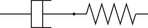 |
22% | 100% |
 |
23% | 97% |  |
21% | 96% |
The advantage of using analytical derivatives becomes more pronounced, particularly for complex rheological models, where simulations using analytical derivatives are significantly faster. This finding aligns with the results obtained by Rothe and Hartmann [12], where the comparison between numerical and analytical tangents with tangents obtained by automatic differentiation showed less significant differences than observed here. The reason for this discrepancy could be attributed to the presence of nested numerical tangents in the presented implementation, which are computationally expensive but not necessary in classic implementations like the one in Rothe and Hartmann [12].
An additional benefit of analytical tangents is their stability, especially when nested tangents are required (see Table 2), as the accuracy of numerical tangents decreases with each nested level. While a difference of 3 or 4% may seem insignificant, it can accumulate to hundreds of iterations over the course of the entire simulation.
However, a disadvantage of analytical tangents is the requirement for deriving the analytical tangents, when implementing new material laws or new rheological elements.
6 SUMMARY AND OUTLOOK
In this paper, an algorithm was presented for automatic simulation of the stress response in rheological models. In addition, a method was demonstrated for implementing analytical tangents for these rheological models and automatically computing them. This approach enhances the stability of the simulation, particularly for deeply nested models, and significantly reduces the simulation time.
The next objective is to extend the algorithm to handle rheological models with an arbitrary number of elements in serial connections.
ACKNOWLEDGMENTS
Open access funding enabled and organized by Projekt DEAL.