Volume 23, Issue 4 e202300107
RESEARCH ARTICLE
Open Access

Extension of a shell-like RVE model to represent transverse shear effects in textile reinforced composites

Omar Khattabi

Corresponding Author

Omar Khattabi

Chair of Solid Mechanics, Chemnitz University of Technology, Chemnitz, Germany

Correspondence

Omar Khattabi, Chair of Solid Mechanics, Chemnitz University of Technology, Reichenhainer Str. 70, 09126 Chemnitz, Germany.

Email: [email protected]

Search for more papers by this author
Ralf Landgraf

Ralf Landgraf

Chair of Solid Mechanics, Chemnitz University of Technology, Chemnitz, Germany

Search for more papers by this author
Jörn Ihlemann

Jörn Ihlemann

Chair of Solid Mechanics, Chemnitz University of Technology, Chemnitz, Germany

Search for more papers by this author
First published: 04 December 2023

Abstract

Textile reinforcements have long been used in shell-like components like tires, belts, hoses and, in particular, air spring bellows. These bellows consist of a certain number of cords embedded in soft rubber, resulting in high membrane stiffness to absorb tensile forces and low resistance to changes in curvature. The embedded cords are produced by twisting multifilament yarns. Modelling and simulation of bellows is a challenging task. Thereby, the complex internal geometry, large deformations as well as the strongly anisotropic and nonlinear material behavior have to be taken into account in a computationally efficient manner. One approach is the application of multiscale analyses in conjunction with representative volume elements (RVE). Within this study, a through-thickness RVE based on in-plane periodic microstructures is applied. The local behavior of the cords is represented by an anisotropic constitutive model that regards directions and mechanical properties of filaments, which result from previous cord twisting simulations. In this contribution, an extension of the classical periodic boundary conditions (PBC) is presented, which considers curvature, pressure load, and, in particular, transverse shear. The RVE is used to simulate the stresses and strains in cord-rubber composites under realistic load conditions. Moreover, it is employed for homogenizing the mechanical behavior and, thus, for developing a suitable constitutive model for shells.

1 INTRODUCTION

Air spring bellows feature a highly complex internal geometry and are characterized by strong anisotropic, nonlinear material behavior, generally large deformations, and contact. The main objective is to provide novel high-resolution models that account for these characteristics for the structural mechanical simulation of air springs. Consequently, the models have to be both efficient and realistic. Figure 1 illustrates a cross-ply reinforced bellows. The rubber matrix contains two layers of textile cords, which are oriented at the angle α relative to the axial direction and are significantly stiffer than the cord matrix. However, the cord owns a complex geometry and filament structure. The filament structure plays an important role in determining the stiffness properties of the cord and, consequently, the resulting stiffness properties of the composite. This composite structure allows for the absorption of significant membrane forces, which are crucial for the load-carrying capacity of the air spring. Due to the dominant influence of the rubber matrix, the composite remains highly flexible against bending. Over the past years, many finite element models have been developed for cord-rubber composites. Frequently, these models use simplifications to deal with the complex structure of the cord, its anisotropic behavior, significant large deformations, or the challenging discretization of the composite [1]. For instance, shell elements or rebar models are often employed to analyze the overall behavior of the component. However, these models are not capable of accurately determining local results such as stresses or strains. For such an evaluation, microstructural modelling is required, considering a representative volume element (RVE). These models have the advantage of providing a larger number of elements to resolve the large gradients near the interface. The challenge with these models lies in formulating the macroscopic boundary conditions in such a way that an efficient analysis of real loads on shell-like structures is enabled, while minimizing disruptions caused by boundary effects. Typical loadings on those structures are curvatures, membrane deformations, transversal shear, and pressure loads. The shell-like RVE can capture important features such as microscopic geometric structures and material properties that influence the overall behavior of the system. By analyzing such an RVE, valuable insights into the behavior of the larger system can be gained without the need to model the entire structure or material. Thus, the RVE can be replaced by a shell element of the same physical properties. This procedure is called homogenization. With the aid of a submodel, which is surrounded by an elastomer layer, the results in the interface region can be further enhanced. The boundary conditions of the submodel are derived from the macroscopic simulation of the RVE.

Details are in the caption following the image
Representation of a rolling lobe air spring (left) as well as microscopic images of bellows cross-sections (right) showing the cross-section and longitudinal view of the cords [2].

2 HOMOGENIZATION

Homogenization is efficiently applied in multiscale modelling when the complexity of the geometric and mechanical microstructure is too challenging to be handled by other conventional modelling techniques. In order to describe the behavior of composite materials, there are three methods of homogenization. The first method is analytical homogenization, followed by numerical homogenization techniques, such as fast Fourier transformation (FFT)-based homogenization for obtaining effective properties in linear elasticity and conductivity problems. Thus, this method is not suitable for arbitrary microscale material behavior, including physically nonlinear and time dependent behavior [3]. The last method is computational homogenization, which represents an effective method for incorporating multiscale hierarchies into computational models. The basic idea behind computational homogenization is to couple two finite element models ( FE 2 $\text{FE}^2$ ) by solving a microscale boundary value problem at the integration points of the macroscale model. However, the main challenge of this approach is the high computational cost, which requires additional efforts to explore strategies for reducing the computational costs. The theory of shell computation homogenization is proposed by [4] and [5]. The aim of this paper is to develop a shell-like RVE for highly loaded thin cord-elastomer composites that is capable of simulating not only membrane deformations, large curvatures, and internal pressure but also transverse shear. Two homogenization techniques are implemented and compared in order to identify the optimal approach for defining the periodic boundary conditions (PBC). The first technique, proposed by [4], represents a second-order computational homogenization framework of thin shells, as an extension of the classical first-order computational homogenization framework introduced by [6]. This technique is presented in detail in Section 2.2 of the paper. The second technique, proposed by [1], extends the classical first-order PBC to allow for rigid body rotation of the material line elements at the periodic surfaces of the RVE. In the context of this work, the second technique is further extended to incorporate transverse shear deformation. This technique is explained in Section 2.3.

2.1 Macroscale mindlin-reissner kinematics

The Mindlin-Reissner theory, also known as the first-order shear deformation theory, employs a linear approximation for the displacements of the cross-section, as illustrated in Figure 2. In contrast to the Kirchhoff-Love plate theory, in which a cross-section perpendicular to the plate's midplane remains straight and perpendicular after deformation, the Mindlin-Reissner concept allows for a rotation of the cross-section while maintaining its straightness. The number of bars under the tensor symbol represents the tensor's order. For instance, vectors are represented with a single bar, while second-order tensors are denoted with two bars. Figure 2 shows the trajectory of an arbitrary material point. The position vectors r ̲ ${\underline{\widetilde{r}}}$ and r ̲ $\underline{r}$ represent the point's location in the reference and current configurations, respectively. Although both vectors are expressed in the global coordinate system e ̲ i $\underline{e}_{i}$ , they can also be described using local curvilinear coordinates ( ξ 1 , ξ 2 , ξ 3 ) $({\xi ^{1},\xi ^{2},\xi ^{3}})$ . The coordinates ξ α $\xi ^{\alpha }$ correspond to the mid-surface of the shell continuum with α = 1 , 2 $\alpha = 1,2$ , with the associated tensor being depicted in bold. Meanwhile, the coordinate ξ3 represents the direction transverse to the mid-surface. In the reference configuration, the position vector of any material point can be linearly approximated as follows [7].
r ̲ ξ α , ξ 3 = r ̲ ξ α + ξ 3 d ̲ ξ α with r ̲ , α = g ̲ α + ξ 3 d ̲ , α and r ̲ , 3 = d ̲ r ̲ ξ α , ξ 3 = r ̲ ξ α + ξ 3 d ̲ ξ α with r ̲ , α = g ̲ α + ξ 3 d ̲ , α and r ̲ , 3 = d ̲ $$\begin{equation} \def\eqcellsep{&}\begin{array}{llll}\underline{\widetilde{r}}{\left(\xi ^{\alpha },\xi ^{3}\right)}&=\underline{\widetilde{r}}{}_{\parallel }{\left(\xi ^\alpha \right)}+\xi ^3\, {\underline{\widetilde{d}}}{\left(\xi ^{\alpha }\right)} &\quad \text{with} \quad {\underline{\widetilde{r}}}_{,\alpha } = \underline{\widetilde{g}}{}_{\alpha } + \xi ^3\, \underline{{\it {d}}}_{,\alpha } &\quad \text{and} \quad {\underline{\widetilde{r}}}_{,3}={\underline{\widetilde{d}}}\\[3pt] {\underline{r}}{\left(\xi ^{\alpha },\xi ^{3}\right)}&={\underline{r}}{}_{\parallel }{\left(\xi ^{\alpha }\right)}+\xi ^{3}\, {\underline{d}}{\left(\xi ^{\alpha }\right)} &\quad \text{with} \quad {\underline{r}_{,\alpha }} = {\underline{g}_{\alpha }} + \xi ^{3}\, {\underline{d}_{,\alpha }} &\quad \text{and} \quad {\underline{r}_{,3}}={\underline{d}} \end{array} \end{equation}$$ (1)
Details are in the caption following the image
Mindlin-Reissner shell: reference state (left) and deformed state (right).
The operators ( * ) , α $(\ast )_{,\alpha }$ and (*), 3 are defined as the partial derivatives of (*) with respect to ξ α $\xi ^{\alpha }$ and ξ3, respectively. In the current configuration, the director d ̲ $\underline{d}$ is rotated with respect to the original director d ̲ ${\underline{\widetilde{d}}}$ due to two factors: transverse shear φ λ $\varphi _\lambda$ and rotation of the reference plane by the angle φ k $\varphi _k$ . The transverse shear deformation causes a rotation of the director along the thickness of the material, while the rotation of the reference plane is associated with the curvature of the structure. The transport of a material line element from the undeformed to the deformed configuration is described by the following operator:
d r ̲ = F ̲ ̲ · d r ̲ with F ̲ ̲ = g ̲ α g ̲ α + ξ 3 d ̲ , α g ̲ α + d ̲ d ̲ $$\begin{align} \mathrm{d}{\underline{r}} =\underline{\underline{F}} \cdot \mathrm{d}{\underline{\widetilde{r}}} \quad \text{with} \quad \underline{\underline{F}} = {\underline{g}_{\alpha }}\otimes \underline{\widetilde{g}}^{\alpha } + \xi ^{3}\,{\underline{d}_{,\alpha }}\otimes \underline{\widetilde{g}}^{\alpha }+{\underline{d}}\otimes {\underline{\widetilde{d}}} \end{align}$$ (2)
The macroscale deformation gradient tensor F ̲ ̲ $\underline{\underline{F}}$ of the three-dimensional continuum is approximated using the first-order Mindlin-Reissner theory with F ̲ ̲ = g ̲ α g ̲ α $\underline{\underline{\bm {F}}}={\underline{g}_{\alpha }}\otimes \underline{\widetilde{g}}{}^{\alpha }$ as the in-plane deformation gradient tensor of the reference surface, which corresponds to the membrane deformation tensor in shell theories. Moreover, K ̲ ̲ = d ̲ , α g ̲ α $\underline{\underline{\bm {K}}}=\underline{\widetilde{d}}_{,\alpha }\otimes \underline{\widetilde{g}}{}^{\alpha }$ is the curvature tensor, and d ̲ $\underline{d}$ represents the in-plane transverse shear. Additionally, in accordance with classical shell theories, an infinitesimal rotation description is employed for the in-plane deformation of the director, effectively restricting the main of curvature to a small value of H = 1 2 K ̲ ̲ · F ̲ ̲ 1 1 $H=\tfrac{1}{2}{\underline{\underline{\bm {K}}}}\cdot {\underline{\underline{\bm {F}}}^{-1}}\ll 1$ . The shell strains are obtained based on the assumed kinematics stated in assumption (2) and can be defined as follows [7]
h ̲ ̲ = 1 2 ln ( ( F ̲ ̲ · F ̲ ̲ T ) ) , κ ̲ ̲ = K ̲ ̲ · F ̲ ̲ 1 F ̲ ̲ T · K ̲ ̲ 0 · F ̲ ̲ 1 , γ ̲ = g ̲ α · d ̲ g ̲ α · d ̲ g ̲ α , $$\begin{equation} \def\eqcellsep{&}\begin{array}{lll}\underline{\underline{\bm {h}}} = \dfrac{1}{2}\ln ((\underline{\underline{\bm {F}}}\cdot \underline{\underline{\bm {F}}}^T)) \quad , & \underline{\underline{\bm {\kappa }}} = \underline{\underline{\bm {K}}}\cdot \underline{\underline{\bm {F}}}^{-1}-\underline{\underline{\bm {F}}}^{-T}\cdot \underline{\underline{\bm {K}}}{}_{0}\cdot \underline{\underline{\bm {F}}}^{-1}\quad , & {\underline{\gamma }} = {\left({\underline{g}_{\alpha }}\cdot {\underline{d}}-\underline{\widetilde{g}}_{\alpha }\cdot \underline{\widetilde{d}}\,\right)}\,\underline{g}^{\alpha }, \end{array} \end{equation}$$ (3)
where h ̲ ̲ ${\underline{\underline{\bm {h}}}}$ is a Hencky-tensor of the membrane deformation, κ ̲ ̲ ${\underline{\underline{\bm {\kappa }}}}$ is denotes a symmetric relative curvature tensor, γ ̲ ${\underline{\gamma }}$ represents the transverse shear strains, and ln ( ( ) ) $\ln ((\cdots ))$ denotes the tensorial natural logarithmic function. The membrane forces are quantified as N α β ${{\it {N}}{}_{\alpha \beta }}$ in [N mm] units, the bending moments are symbolized as M α β ${{\it {M}}{}_{\alpha \beta }}$ in [N mm2] units, and the shear forces are indicated as S α ${{\it {S}}{}_{\alpha }}$ in [N mm] units, with their expressions as follows
N α β = h σ α β d ξ 3 , M α β = h ξ 3 σ α β d ξ 3 , S α = h σ 3 α d ξ 3 , $$\begin{equation} {{\it {N}}{}_{\alpha \beta }} = \int _{h} {{\it {\sigma }}{}_{\alpha \beta }}\, \mathrm{d}\xi ^{3} \quad ,\quad {{\it {M}}{}_{\alpha \beta }} = \int _{h} \xi ^{3}\,{{\it {\sigma }}{}_{\alpha \beta }}\, \mathrm{d}\xi ^{3} \quad ,\quad {{\it {S}}{}_{\alpha }} = \int _{h} {{\it {\sigma }}{}_{3\alpha }}\, \mathrm{d}\xi ^{3} \,, \end{equation}$$ (4)
Here, h represents the thickness of the shell. To define the nonlinear mechanical behavior of a shell section in terms of generalized section quantities using the ABAQUS subroutine UGENS, the force array [Ni] and strain array [Ei] are used. In these arrays, the direct membrane terms are stored first, followed by the shear membrane term, the direct and shear bending terms, and then the transverse shear components, as defined in Equation (5). The number of entries in these arrays depends on the specific element type, as only the active components are stored.
[ N i ] = N 11 , N 22 , 1 2 ( N 12 + N 21 ) , M 11 , M 22 , 1 2 ( M 12 + M 21 ) , S 1 , S 2 [ E i ] = h 11 , h 22 , 2 h 12 , κ 11 , κ 22 , 2 κ 12 , γ 1 , γ 2 $$\begin{align} \def\eqcellsep{&}\begin{array}{ll} {[\bm{N}_i]} &= {\left[N_{11},N_{22},\dfrac{1}{2}(N_{12}+N_{21}),M_{11},M_{22},\dfrac{1}{2}(M_{12}+M_{21}),S_{1},S_{2}\right]}\\[3pt] {[\bm{E}_i]} &={\left[h_{11},h_{22},2\,h_{12},\kappa _{11},\kappa _{22},2\,\kappa _{12},\gamma _{1},\gamma _{2}\right]}\\[3pt] \end{array} \end{align}$$ (5)
The linearized constitutive relations that align with the macroscopic framework can be expressed as follows
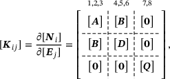
image(6)
where the macroscopic constitutive tangents of a shell element are captured by an 8 × 8 stiffness matrix [ K i j $\bm{K}_{ij}$ ]. This matrix can be decomposed into four distinct parts. The first part [A] is the so-called membrane stiffness, the second part [D] represents the plate stiffness and the mixed derivatives [B] correspond to coupling stiffnesses, accounting for the coupling between in-plane and out-of-plane deformations. The last part [Q] represent the transverse shear stiffness.

2.2 Microscale projection: Second-order homogenization

The transition from macro- to microscales involves averaging relationships that establish the boundary conditions for a microstructural RVE. These boundary conditions impose the macroscopic quantities, specifically the generalized strains F ̲ ̲ ${\underline{\underline{\bm {F}}}}$ , K ̲ ̲ ${\underline{\underline{\bm {K}}}}$ , and d ̲ ${\underline{d}}$ . This transition departs from the formulation (expressed in Equation (2)) for the material line element within a shell at the in-plane level. In order to consider the influence of a local fine-scale microstructure and its associated displacement field, a microfluctuation field w ̲ m ${\underline{w}}_{m}$ is introduced and superimposed onto the macroscopic displacement field. However, the transition is only applied to the surfaces of the microstructural RVE that have normal vectors n ̲ α ${\underline{\widetilde{n}}}_{\alpha }$ tangential to the midplane. Figure 3 provides a representation of these surfaces and their orientation relative to the midplane. On the other hand, the surfaces of the RVE that have a normal vector in the thickness direction remain unconstrained. Here, the displacement vector u ̲ $\underline{u}$ and the average three-dimensional macroscale displacement gradient H ̲ ̲ ${\underline{\underline{H}}}$ are relevant. Consequently, the PBC couple the displacements of specific pairs of points. The Taylor expansion of the macroscopic field is
Δ u ̲ = H ̲ ̲ · Δ r ̲ + w ̲ m with H ̲ ̲ = F ̲ ̲ I ̲ ̲ + ξ 3 K ̲ ̲ + d ̲ d ̲ . $$\begin{align} \Delta \underline{u} = {\underline{\underline{H}}}\cdot \Delta \underline{\widetilde{r}} + {\underline{w}}_{m} \quad \text{with} \quad {\underline{\underline{H}}} = \underline{\underline{F}}-{\underline{\underline{I}}} + \xi ^{3}\,\underline{\underline{K}}+ {\underline{d}}\otimes {\underline{\widetilde{d}}}{} \,. \end{align}$$ (7)
Details are in the caption following the image
Second-order RVE. RVE, representative volume elements.

The displacements of the cross-section are linearly approximated, which leads to deviations when the cross-section undergoes large rotations.

2.3 Microscale projection: Rotation-based homogenization
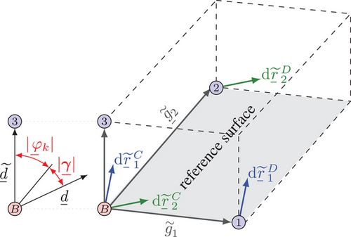
In the case of an air spring bellows, the curvatures are dominant and highly significant. Therefore, it is of great importance to develop an RVE-model with rotation-based PBC that is capable of simulating the significant rotations of the cross-section. Thereby, the modification of the PBC should be done without violating the assumptions of the Mindlin-Reissner shell theory, in order to maintain information exchange between the macro and micro FE-models. Henceforth, side surfaces of the rotation based RVE are divided into so-called “control surfaces” and “dependent surfaces”, where each dependent surface lies opposite to a corresponding control surface. To aid in comprehension, the corresponding material line elements at the control and dependent surfaces are represented as d r ̲ α C $\mathrm{d}\underline{r}^{C}_{\alpha }$ and d r ̲ α D $\mathrm{d}\underline{r}^{D}_{\alpha }$ , respectively, as shown in the Figure 4. The PBCs ensure that two opposing surfaces are identical, with the exception of a rigid body rotation of the material line elements, which depends on membrane deformation F ̲ ̲ ${\underline{\underline{\bm {F}}}}$ and curvature tensor K ̲ ̲ ${\underline{\underline{\bm {K}}}}$ . This leads to the constraint (8). By enforcing this constraint, the behavior and deformation of the dependent surfaces are directly linked to those of the corresponding control surfaces, preserving the periodicity and allowing for the analysis or modeling of periodic structures. However, to extend the PBC to include transverse shear γ ̲ ${\underline{\gamma }}$ , the director (only the edge between 3 and B) is rotated using a rotation tensor Q ̲ ̲ $\underline{\underline{Q}}$ , which determines a rotation angle and a rotation axis using the Euler-Rodrigues formula.
d r ̲ α D = Δ R ̲ ̲ α · d r ̲ α C and d ̲ = Q ̲ ̲ φ ̲ k , γ ̲ · d ̲ with Δ R ̲ ̲ α φ ̲ k = exp g ̲ α × d ̲ × K ̲ ̲ · F ̲ ̲ 1 $$\begin{align} \mathrm{d}{\underline{r}^{D}_{\alpha }} =\Delta {\underline{\underline{R}}{}_{\alpha }}\cdot \mathrm{d}{\underline{r}^{C}_{\alpha }} \quad \text{and}\quad {\underline{d}} = {\underline{\underline{Q}}}{\left(\underline{\varphi }{}_{k},\underline{\gamma }\right)}\cdot {\underline{\widetilde{d}}} \quad \text{with}\quad \Delta {\underline{\underline{R}}{}_{\alpha }}{\left(\underline{\varphi }{}_{k}\right)}=\exp \,{\left({\left({\underline{g}_{\alpha }} \times {\left({\underline{\widetilde{d}}}\times {\underline{\underline{\bm {K}}}}\cdot {\underline{\underline{\bm {F}}}^{-1}}\right)}\,\right)}\right)} \end{align}$$ (8)
Details are in the caption following the image
Rotation-based RVE. RVE, representative volume elements.

It is important to emphasize that only surfaces with a Gaussian curvature det [ K α β ] = 0 $ \mathrm{det}[{\it {K}_{\alpha \beta }}] = 0$ are considered as so-called developable surfaces. This means that the curved surface can be flattened without distortion. Please note that the sphere is the only closed surface with a constant Gaussian curvature. In general, undesired surface effects increase with increasing Gaussian curvature. Therefore, either small RVEs of highly curved surfaces or large RVEs of slightly curved surfaces can be analyzed with negligible surface effects. In the case of an air spring, the curvature of the rolling lobe is large compared to the curvature in the circumferential direction. Hence, the highly loaded areas can be modeled as a parabolic RVE.

2.4 Implementation

ABAQUS provides a user-defined subroutine called the multi-point constraint (MPC), which allows the imposition of nonlinear constraints. In order to specify the macroscale displacement gradient in a local orthogonal coordinate system e ̲ i ${\underline{e}}_{i}$ , three additional pilot nodes P α ( α = 1 , 2 ) ${P}_{\alpha}(\alpha =1,2)$ in-plane and P3 out-of-plane are introduced (see Figure 3), which are not physically connected to the RVE. The displacement degrees of freedom U P α β $U_{P\alpha _{\beta }}$ and U P 3 β $U_{P3_\beta }$ (with U P α 3 = U P 3 3 = 0 $U_{P\alpha _3}=U_{P3_3}=0$ ) are utilized to define the coefficients of the membrane tensor F ̲ ̲ $\underline{\underline{F}}$ and the transverse shear λ ̲ = d α e ̲ α $\underline{\bm {\lambda }} = d_\alpha \,{\underline{e}}_{\alpha }$ , respectively. Conversely, the rotational degrees of freedom U R P α β $UR_{P\alpha _{\beta }}$ (with U R P α 3 = U R P 3 i = 0 $UR_{P\alpha _3}=UR_{P3_i}=0$ ) are employed to determine the coefficients of the curvature tensor K ̲ ̲ $\underline{\underline{K}}$ .
[ F α β ] = U P 1 1 + 1 U P 1 2 U P 2 1 U P 2 2 + 1 [ K α β ] = U R P 1 2 U R P 1 1 U R P 2 2 U R P 2 1 [ λ α ] = U P 3 1 U P 3 2 $$\begin{equation} [\bm{F}{}_{\alpha \beta}]=\left[ \def\eqcellsep{&}\begin{array}{cc}{U}_{P{1}_{1}}+1& {U}_{P{1}_{2}}\\ {U}_{P{2}_{1}}& {U}_{P{2}_{2}}+1\end{array} \right]\hspace*{2em}[\bm{K}{}_{\alpha \beta}]=\left[ \def\eqcellsep{&}\begin{array}{cc}U{R}_{P{1}_{2}}& U{R}_{P{1}_{1}}\\ U{R}_{P{2}_{2}}& U{R}_{P{2}_{1}}\end{array} \right]\hspace*{2em}[\bm{\lambda}{}_{\alpha}]=\left[ \def\eqcellsep{&}\begin{array}{c}{U}_{P{3}_{1}}\\ {U}_{P{3}_{2}}\end{array} \right] \end{equation}$$ (9)

3 NUMERICAL RESULTS

3.1 Verification of surface effects and validation

To verify the surface effects, multiple homogeneous second-order RVEs are connected in series. These RVEs are defined by dimensions specified as N [ l × w × h ] $N\,[l\times w \times h]$ , with the number of these RVEs denoted as N, and each having defined length (l), width (w), and thickness (h). These RVEs are loaded with a high curvature of K 11 = 0.4 mm 1 $K_{11}=0.4\,\mathrm{mm^{-1}}$ . The surface effects refer to disturbances in the peripheral regions of the RVE. On the left side of the illustration 5 (the first image from the left), it is clearly evident that changes in the von Mises stress distribution occur not only in the thickness direction but also in other coordinate directions, indicating disturbances in the peripheral areas. When the RVE is reduced in size (as seen in the third image from the left), the disturbances in the peripheral region decrease despite constant curvature. This becomes particularly evident when the stress distribution changes exclusively in the thickness direction. From this, the following conclusion can be drawn: When analyzing a small RVE with significant curvature, the curvature is indeed significant, but the RVEs are small enough to assume that surface effects are relatively negligible. The smaller the RVE, the more the surface effect is reduced until it converges to a free surface effect. In contrast, when examining large RVEs with minimal curvature, the curvature is less pronounced, but the RVEs are large enough to justify the assumption that surface effects are negligible. In the case of a rotation-based RVE, the stress distribution is only free from thickness any surface effects in the parabolic scenario, regardless of the size of the RVE, as depicted in Figure 6 on the left. This is due to the strict constraints in Equation (8). This emphasizes the statements of the theorems by Minding and Liebmann, which explain the surface effects in elliptical and hyperbolic structures. Only surfaces with a Gaussian curvature of zero are considered “developable”, meaning that the curved surface can be flattened without distortion.

Details are in the caption following the image
Von Mises stress in RVEs connected in series of different sizes. RVE, representative volume elements.
Details are in the caption following the image
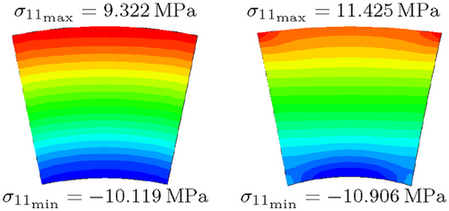
In-plane stress σ11 distribution resulting from the simple bending of a rotation-based RVE (left), and of a second-order RVE (right). RVE, representative volume elements.

In order to prove the correct implementation of the constraints and the validity of the homogenization, a homogeneous FE-plate made of elastomer is considered. Initially, a FE-plate with dimensions of 10 × 40 × 1 mm 3 $10\times 40\times 1 \,\mathrm{mm^{3}}$ for length, width, and thickness is modeled, using volume elements (5 elements in the thickness direction). The plate is assigned a soft isotropic material with Hooke's parameters E = 42 MPa , ν = 0.4 $E = 42\,\mathrm{MPa},\; \nu = 0.4$ , and a curvature of K 11 = 0.4 mm 1 $K_{11} = 0.4\,\mathrm{mm^{-1}}$ is applied. The results of the macroscopic simulation show at a specific location the maximum normal stress in the tensile region of σ 11 max = 9.32 MPa $\sigma _{{11}\mathrm{max}}=9.32\,\mathrm{MPa}$ (on the upper surface) and the minimum normal stress of σ 11 min = 10.12 MPa $\sigma _{{11}\mathrm{min}}=-10.12\,\mathrm{MPa}$ in the compressive region (on the lower surface). At the same location, an RVE with dimensions of 1 × 1 × 1 mm 3 $1\times 1\times 1\,\mathrm{mm^{3}}$ is extracted, and the same material and boundary condition parameters are applied. The results of the microscopic simulation of the RVE using both methods are presented in Figure 6. It is shown that the rotation-based RVE provides more accurate results, and the small differences observed are due to numerical differentiation and can be disregarded when using a fine mesh. Instead, the second-order RVE exhibits some deviation, which diminishes as the size is reduced. It is shown that the rotation-based RVE provides more accurate results, and the small deviation in results between the FE plate and the RVE is attributed to numerical differentiation and can be disregarded when using a fine mesh. Instead, the second-order RVE exhibits some deviation, which diminishes as the size of RVE is reduced.

3.2 Cross-layer reinforced composites of an air spring

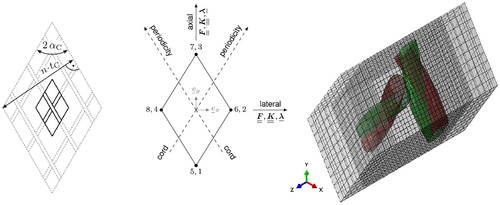
In this section, shell-like rotation-based RVEs for cord-elastomer composites with two intersecting reinforcement layers are considered. The objective is to analyze the locale stresses (localization) in the composite under realistic loading conditions that occur in a component such as an air spring. This aims to enable efficient optimization of cord-elastomer composites, including their durability, under realistic conditions. Figure 7 (left) shows the geometry of an undeformed air spring bellows with its dimensions in a top view. The RVEs represent sections of the bellows with different periodicity and loading directions. Although the initial geometry of many air spring bellows is cylindrical, the RVEs are assumed to be initially straight due to the large radius compared to the bellows thickness and the high number of cords n. The parameters of the cross-layer reinforced composite are cord angle α C $\alpha _C$ , the thickness of the composite h, the spacing of the cords t C $t_C$ , and the relative position of the cords in the thickness direction. The RVE features a structured mesh with C3D8H hybrid elements, and the material model assigned to each integration point is assumed to be influenced by its corresponding material region. A hyperelastic model is chosen for the rubber matrix. In particular, the strain energy potential of Neo-Hookean type is used, which is split into deviatoric and volumetric contributions. The second material region that needs to be considered is the cord, which has a filament structure. The cord bundle is considered to possess transversely isotropic behavior with the preferred direction represented by t ̲ F $\underline{t}_F$ . The total strain energy potential is composed of an anisotropic part and an isotropic part that accounts for shear and volumetric deformations [1]. The next step involves developing a global FE model in ABAQUS using the rebar formulation. In this context, the global model refers to an FE model of the air spring that does not rely on any assumed symmetries. The aim of the global model is to accurately capture all typical macroscopic deformation modes present in the air spring bellows, enabling their transfer to the RVE.
Details are in the caption following the image
Cross-ply RVEs as sections of air spring bellows. RVE, representative volume elements.

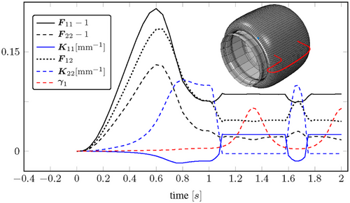
These deformation modes specifically include membrane deformation, curvatures, and transverse shear effects occurring within the matrix between two cord layers (see, ref. [8]), as illustrated in Figure 8. A transfer of the macroscopic deformations to the RVE as PBC allows for a more precise analysis of the local stress distribution. However, the use of multiphase elements inevitably entails a loss of information concerning the interface. Since the interface between the cords and the elastomer often represents preferred locations for crack initiation and, consequently, for later component failure, the analysis of stress in this region is of particular interest. One way to significantly improve the quality of results near the interface is through the application of submodeling techniques. Figure 9 illustrates the distribution of maximum logarithmic strain in both the RVE and the submodel. Based on the simulations, it has been observed that the primary influence in changing the cord angle is a result of the combined effects of curvature and transverse shear. This interaction leads to a significant shearing of the elastomer layer located between the cord layers. The subsequent step involves calculating an effective shell stiffness using a second-order RVE, as depicted in Figure 9. This calculation is necessary for homogenization the effective mechanical behavior of the corresponding shell element and, thus, developing an appropriate constitutive model.
Details are in the caption following the image
the local macroscopic deformation modes in a rebar model.
Details are in the caption following the image
The distribution of maximum logarithmic strain in RVE (left), and in a submodel of a cord, which is coated with an elastomer layer (middle), and effective shell stiffness (right). RVE, representative volume elements.

Additionally, all contributions highlighted in red appear as discretization errors. Besides the tension-torsion coupling, the coupling between bending and shearing is particularly interesting. Due to the curvature of the RVE, tension and compression sides are formed. Instead of simply stretching or compressing, the cords can also change their angle in response.

4 SUMMARY

The rotation-based RVE is expanded to incorporate transverse shear and is highly suitable for localization and accurately analyzing the local stress in cord-elastomer composites. Its effectiveness lies in its ability to simulate significant curvature effects at different sizes without violating the periodicity conditions. For its discretization, a simple structured meshing approach was used, combined with an integration point-wise assignment of material properties, resulting in a suitable FE model for cord-elastomer composites. The loss of information due to the implicitly modeled interface between the materials was compensated for by conducting a subsequent analysis of a submodel of a cord, which is coated with an elastomer layer. However, the rotation-based RVE is unable to simulate arbitrary curvatures in different directions. The curvature tensor must satisfy certain conditions, such as having zero Gaussian curvature, in order to avoid surface effects. In case of non-zero Gaussian curvature, like in air springs, the second-order RVE is perfectly suited for homogenizing the effective properties and coupling with shell elements in FE 2 $\text{FE}^2$ analyses. However, it is important to choose an appropriate size to minimize surface effects.

ACKNOWLEDGMENTS

Open access funding enabled and organized by Projekt DEAL.

      The full text of this article hosted at iucr.org is unavailable due to technical difficulties.