Volume 23, Issue 4 e202300081
RESEARCH ARTICLE
Open Access

A model for the evolution size and composition of olivine crystals

Hendrik Holger Haddenhorst

Corresponding Author

Hendrik Holger Haddenhorst

Institute of Mechanics of Materials, Ruhr-Universität Bochum, Bochum, Germany

Correspondence

Hendrik Holger Haddenhorst, Institute of Mechanics of Materials, Ruhr-Universität Bochum, D-44780 Bochum, Germany.

Email: [email protected]

Search for more papers by this author
Sumit Chakraborty

Sumit Chakraborty

Institute for Geology, Mineralogy and Geophysics, Ruhr-Universität Bochum, Bochum, Germany

Search for more papers by this author
Klaus Hackl

Klaus Hackl

Institute of Mechanics of Materials, Ruhr-Universität Bochum, Bochum, Germany

Search for more papers by this author
First published: 26 October 2023

Abstract

In this proceeding, a material model to describe the evolution of olivine crystals, in particular iron-based Fayalite crystals, which are affected by the diffusion of magnesium ions, is introduced. These crystals are present in magma and understanding their behavior is an important aspect in improving prediction tools for volcanic eruptions. The model describes the development of the dislocation density, the concentration of magnesium over location and time, as well as the development of the size of the crystal over time. We discuss the model and the corresponding parameters. Furthermore, we present a numerical implementation of the model employing the platform Julia as well as a study on the influence of the various model parameters on the results. The results show a clear threshold between stable and unstable crystals.

1 INTRODUCTION

In geosciences, the understanding of the diffusion history of crystals is of significant importance. In the lower magma chambers of volcanoes, olivine crystals are formed. Due to volcanic activity, these olivine are moved into higher magma chambers. In the meanwhile, the olivine crystal grows, thanks to the diffusion of magnesium into the crystal. Due to changes in the surrounding conditions, an olivine crystal might become unstable and recrystallize. In that case, the diffusion history of the crystal is deleted and cannot be traced back any more. The aim of the introduced model is to improve the understanding of this process to predict under which conditions a crystal recrystallizes and under which conditions a crystal remains stable and the diffusion history can be traced back. This idea has been raised by Chakraborty and Dohmen [1].

2 VARIATIONAL MODEL

We employ a variational model to describe the evolution of the radius of an idealized spherical crystal, as well as the evolution of the concentration of magnesium and the dislocation density. The variational formulation is based on the minimization of the sum of the rate of free energy and a dissipation potential with respect to the rate of the internal variables, see for example, Refs. [2, 3].
c ̇ = D 2 c r 2 + 2 r c r , $$\begin{equation} \dot{c} = D {\left(\frac{\partial ^2 c}{\partial r^2}+\frac{2}{r} \frac{\partial c}{\partial r} \right)}, \end{equation}$$ (1)
c ( r , 0 ) = γ c L 2 R 0 + γ R 0 2 r 2 , $$\begin{equation} c(r,0) = \frac{\gamma \, c_\mathrm{L}}{2 R_0 + \gamma R_0^2} \, r^2, \end{equation}$$ (2)
c r ( R , t ) = γ c L c ( R , t ) , $$\begin{equation} \frac{\partial c}{\partial r}(R,t) = \gamma {\left(c_\mathrm{L} - c(R,t) \right)}, \end{equation}$$ (3)
ρ ̇ = 6 α D g ( ρ ) 1 R 2 0 R 2 c r 2 1 r c r r 2 d r , ρ ( 0 ) = ρ 0 , $$\begin{equation} \dot{\rho }= \sqrt {6} \, \alpha D \, g(\rho ) \, \frac{1}{R^2} \int _{0}^{R} {\left| \frac{\partial ^2 c}{\partial r^2} - \frac{1}{r} \frac{\partial c}{\partial r} \right|} r^2 \, \mathrm{d}r, \quad \rho (0) = \rho _0, \end{equation}$$ (4)
R ̇ = M int R Δ G μ b 2 ρ , R ( 0 ) = R 0 $$\begin{equation} \dot{R}=\frac{{M}_{\mathrm{int}}}{R}\left(\mathrm{\Delta}G-\mu {b}^{2}\rho \right),R\operatorname{(}0)={R}_{0} \end{equation}$$ (5)

In this model, R ( t ) $R(t)$ denotes the radius of the idealized spherical crystal, c ( r , t ) $c(r,t)$ denotes the concentration of magnesium, ρ ( t ) $\rho (t)$ denotes the dislocation density, c L $c_L$ denotes the concentration of magnesium within the surrounding melt, D denotes the diffusivity, γ governs the boundary diffusion, α describes the volumetric expansion coefficient of magnesium over iron, g ( ρ ) $g(\rho )$ describes the relation between the evolution of the plastic strain and the evolution of the dislocation density, μ denotes the shear modulus, b denotes the Burgers-vector, M int / R $M_{\mathrm{int}}/R$ is the interface mobility, and Δ G $\Delta G$ denotes the difference of the caloric energies of olivine in solid and liquid state. Here, Equation (1) is the diffusion equation for spherical symmetry, Equation (2) is the initial condition of the distribution of magnesium, Equation (3) is the boundary condition of the diffusion on the edge of the crystal, Equation (4) is the evolution equation of the dislocation density with the initial dislocation density ρ0 and Equation (5) is the evolution equation of the radius with the initial radius R0.

3 NUMERICAL ALGORITHM

3.1 Landau transformation

To implement the model as a numerical algorithm, a Landau transformation has to be performed first. The variable of position r is replaced by a new variable ξ = r / R ( t ) $\xi = r/R(t)$ . This transformation results in the following model:
c ̂ t = R ̇ R ξ c ̂ ξ + D R 2 2 c ̂ ξ 2 + 2 ξ c ̂ ξ , c ̂ ( ξ , 0 ) = γ c L R 0 2 + γ R 0 ξ 2 , c ̂ ξ ( 1 , t ) = γ R c L c ( 1 , t ) , ρ ̇ = 6 α D g ( ρ ) 1 R 2 0 1 2 c ̂ ξ 2 1 ξ c ̂ ξ ξ 2 d ξ , ρ ( 0 ) = ρ 0 , R ̇ = M int R Δ G μ b 2 ρ , R ( 0 ) = R 0 $$\begin{equation} \boxed{ \def\eqcellsep{&}\begin{array}{l}\frac{\partial \hat{c}}{\partial t} = \frac{\dot{R}}{R} \xi \frac{\partial \hat{c}}{\partial \xi } + \frac{D}{R^2} {\left(\frac{\partial ^2 \hat{c}}{\partial \xi ^2} + \frac{2}{\xi } \frac{\partial \hat{c}}{\partial \xi } \right)},\\[3pt] \\[3pt] \hat{c}(\xi ,0) = \frac{\gamma \, c_\mathrm{L} R_0}{2 + \gamma R_0} \, \xi ^2, \\[3pt] \\[3pt] \frac{\partial \hat{c}}{\partial \xi }(1,t) = \gamma R {\left(c_\mathrm{L} - c(1,t) \right)}, \\[3pt] \\[3pt] \displaystyle \dot{\rho }= \sqrt {6} \, \alpha D \, g(\rho ) \, \frac{1}{R^2} \int _{0}^{1} {\left| \frac{\partial ^2 \hat{c}}{\partial \xi ^2} - \frac{1}{\xi } \frac{\partial \hat{c}}{\partial \xi } \right|} \xi ^2 \, \mathrm{d}\xi , \quad \rho (0) = \rho _0, \\[3pt] \\[3pt] \displaystyle \dot{R} =\frac{M_\mathrm{int}}{R} {\left(\Delta G - \mu b^2 \rho \right)}, \quad R(0) = R_0 \end{array} } \end{equation}$$ (6)

3.2 Reduced formulation

In the next step, the new dimensionless variables are introduced.
z = c c L , $$\begin{equation} z = \frac{c}{c_\mathrm{L}}, \end{equation}$$ (7)
which corresponds with the concentration of magnesium c,
y = μ b 2 Δ G ρ , $$\begin{equation} y = \frac{\mu b^2}{\Delta G} \; \rho , \end{equation}$$ (8)
which corresponds with the dislocation density ρ and
x = γ 2 R 2 , $$\begin{equation} x = \gamma ^2 R^2, \end{equation}$$ (9)
which corresponds with the radius of the crystal R.
Furthermore, three new constants are introduced under the assumption that the relation between the evolution of the plastic strain and the evolution of the dislocation density g ( ρ ) $g(\rho )$ is equal to a constant β
A = 2 M int Δ G γ 2 $$\begin{equation} A = 2 M_\mathrm{int} \Delta G \gamma ^2 \end{equation}$$ (10)
B = 6 α D β c L μ b 2 γ 2 Δ G $$\begin{equation} B = \frac{\sqrt {6} \, \alpha D \beta c_\mathrm{L}\mu b^2 \gamma ^2}{\Delta G} \end{equation}$$ (11)
D ¯ = γ 2 D $$\begin{equation} \bar{D} = \gamma ^2 D \end{equation}$$ (12)
The introduction of the constants A, B, and D ¯ $\bar{D}$ has two advantages. The first advantage is that all three constants have the unit [ 1 / time ] $[1/\text{time}]$ , which makes comparisons between the constants more convenient. The second advantage is that the model simplifies further.
z t = 1 x 1 2 ξ x ̇ z ξ + D ¯ 2 z ξ 2 + 2 ξ z ξ , z ( ξ , 0 ) = x 0 2 + x 0 ξ 2 , z ξ ( 1 , t ) = x 1 z ( 1 , t ) , y ̇ = B 1 x 0 1 2 z ξ 2 1 ξ z ξ ξ 2 d ξ , y ( 0 ) = y 0 , x ̇ = A 1 y , x ( 0 ) = x 0 $$\begin{equation} \boxed{ \def\eqcellsep{&}\begin{array}{l}\frac{\partial z}{\partial t} = \frac{1}{x} {\left[\frac{1}{2} \, \xi \dot{x} \frac{\partial z}{\partial \xi } + \bar{D} {\left(\frac{\partial ^2 z}{\partial \xi ^2} + \frac{2}{\xi } \frac{\partial z}{\partial \xi } \right)} \right]},\\[3pt] \\[3pt] z(\xi ,0) = \frac{\sqrt {x_0}}{2 + \sqrt {x_0}} \, \xi ^2,\\[3pt] \\[3pt] \frac{\partial z}{\partial \xi }(1,t) = \sqrt {x} {\left(1 - z(1,t) \right)}, \\[3pt] \\[3pt] \displaystyle \dot{y} = B \, \frac{1}{x} \int _{0}^{1} {\left| \frac{\partial ^2 z}{\partial \xi ^2} - \frac{1}{\xi } \frac{\partial z}{\partial \xi } \right|} \xi ^2 \, \mathrm{d}\xi , \quad y(0) = y_0, \\[3pt] \\[3pt] \displaystyle \dot{x} = A {\left(1 - y \right)}, \quad x(0) = x_0 \end{array} } \end{equation}$$ (13)

As can be seen in Equation (13), the model is now dependent on only four constants, which are the three new constants A, B, and D ¯ $\bar{D}$ and additionally γ. This makes the model both easier to implement and simplifies a parameter study.

3.3 Numerical implementation

The model is discretized using the finite-difference method. The number of steps is N, the number of evaluation points is n = N + 1 $n = N + 1$ , and the step size is d ξ = 1 / N $d\xi = 1/N$ . The indices i go from 0 to n 1 $n-1$ . For the implementation, the initial conditions are defined as
x t = 0 = γ 2 R 0 2 , $$\begin{equation} x_{t=0} = \gamma ^2 R_0^2, \end{equation}$$ (14)
y t = 0 = 0 , $$\begin{equation} y_{t=0} = 0, \end{equation}$$ (15)
z t = 0 , i = x t = 0 2 + x t = 0 ( d ξ · i ) 2 . $$\begin{equation} z_{t=0, i} = \frac{\sqrt {x_{t=0}}}{2 + \sqrt {x_{t=0}}} (d\xi \cdot i)^2. \end{equation}$$ (16)
The steps of the variables are discretized as follows:
d x = A ( 1 y ) $$\begin{equation} dx = A (1 - y) \end{equation}$$ (17)
d y = B x w ( 1 ) + w ( n 2 ) + i = 1 n 2 w ( i ) $$\begin{equation} dy = \frac{B}{x} {\left(w(1)+w(n-2)+\sum _{i=1}^{n-2}w(i)\right)} \end{equation}$$ (18)
with
w ( i ) = d ξ z i 1 2 z i + z i + 1 d ξ 2 1 d ξ · i z i + 1 z i d ξ ( d ξ · i ) 2 $$\begin{equation} w(i) = d\xi {\left|\frac{z_{i-1} - 2z_i + z_{i+1}}{d\xi ^2} - \frac{1}{d\xi \cdot i}\frac{z_{i+1} - z_i}{d\xi }\right|} (d\xi \cdot i)^2 \end{equation}$$ (19)
The value of Equation (19) is considered twice for i = 1 $i = 1$ and i = n 2 $i = n-2$ as Equation (19) is not defined for i = 0 $i = 0$ and i = n 1 $i = n-1$ .
d z i = 1 x 1 2 ( d ξ · i ) d ξ z i + 1 z i d ξ + D ¯ z i 1 2 z i + z i + 1 d ξ 2 2 d ξ · i z i + 1 z i d ξ $$\begin{equation} dz_i = \frac{1}{x} {\left[\frac{1}{2}(d\xi \cdot i) d\xi \frac{z_{i+1} - z_i}{d\xi } + \bar{D}{\left(\frac{z_{i-1} - 2z_i + z_{i+1}}{d\xi ^2} - \frac{2}{d\xi \cdot i} \frac{z_{i+1} - z_i}{d\xi }\right)} \right]} \end{equation}$$ (20)

The equations are implemented in the programming language Julia and solved with the package DifferentialEquations.jl [4].

3.4 Parameter study

As the formulation of the model in Equation (13) is still dependent on four parameters, a parameter study is executed next. The differential equation is solved repeatedly with randomized input parameters. The investigated parameter ranges are 10 m 1 γ 10 3 m 1 $10 \,\mathrm{m}^{-1} \le \gamma \le 10^3 \,\mathrm{m}^{-1}$ , 10 6 m 2 s 1 γ 2 A 10 15 m 2 s 1 γ 2 $10^{-6} \,\mathrm{m}^2 \,\mathrm{s}^{-1} \gamma ^2 \le A \le 10^{-15} \,\mathrm{m}^2 \,\mathrm{s}^{-1} \gamma ^2$ , 10 6 m 2 s 1 γ 2 B 10 15 m 2 s 1 γ 2 $10^{-6} \,\mathrm{m}^2 \,\mathrm{s}^{-1} \gamma ^2 \le B \le 10^{-15} \,\mathrm{m}^2 \,\mathrm{s}^{-1} \gamma ^2$ , and 10 12 m 2 s 1 γ 2 D ¯ 10 20 m 2 s 1 γ 2 $10^{-12} \,\mathrm{m}^2 \,\mathrm{s}^{-1} \gamma ^2 \le \bar{D} \le 10^{-20} \,\mathrm{m}^2 \,\mathrm{s}^{-1} \gamma ^2$ . These input parameters are used with the results to train an Artificial Neural Network in Python using the keras package [5]. This Artificial Neural Network is then used to interpolate further parameter combinations.

4 NUMERICAL RESULTS

4.1 Numerical model

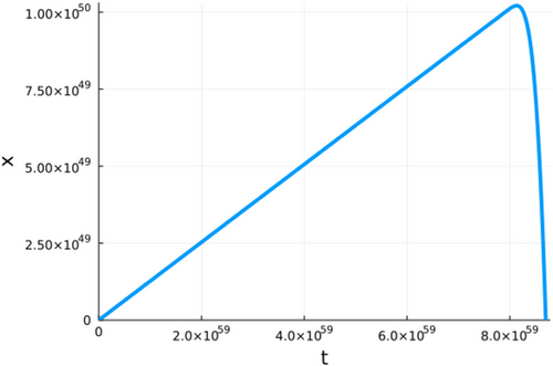
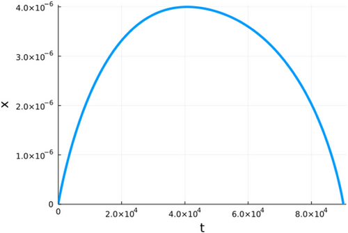
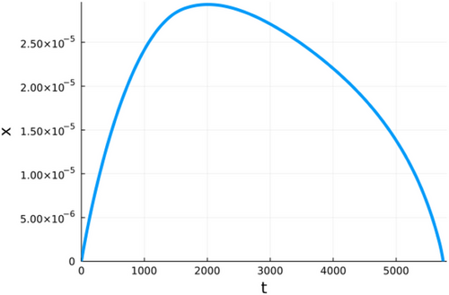
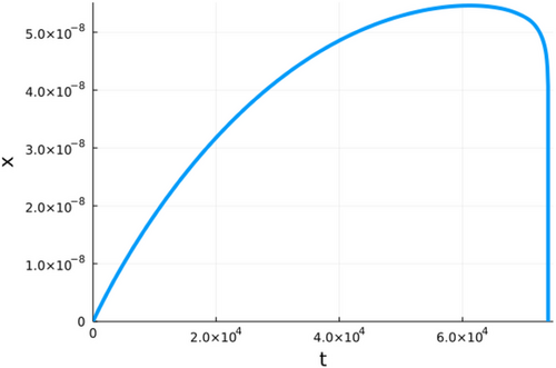
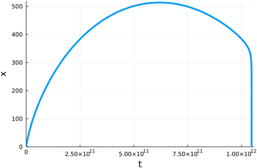
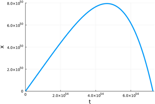
Figures 1-6 show different examples of plots of the size x over time for different parameter combinations. All plots show a constant growth phase at the beginning. After the maximum is reached, the crystal starts shrinking again until the size goes back to 0. At this point, the crystal would recrystallize. It can be observed though that the shapes of the evolutions are significantly different from plot to plot. The plots in Figures 2 and 5 reach their respective maximums relative to their points of failure a lot later than the other plots, while the plot in Figure 4 reaches its maximum size quite early and then shrinks slowly. Furthermore, the axes in the plots have significantly different magnitudes. The most extreme values XMax for the size x can be seen in the plot in Figure 1 with a magnitude of 1050 and in Figure 5 with a magnitude of 10−8. While a magnitude of 1050 can be considered unrealistically large, a magnitude of 10−8 can be considered unrealistically small. With regards to the time of failure Tfailure, there is a similar picture. The most extreme examples in this case are the plot in Figure 2 with a magnitude of 1059 s and plot in Figure 4 with a magnitude of 103 s. Again a magnitude of 1059 s can be considered unrealistically large. On the other hand, a magnitude 103 s, in the case of this plot the exact time of failure is 5.747000 · 103 s, seems realistic in an experimental setting. Generally speaking, crystals with extremely large values for both the maximum size and time of failure can be considered stable in the real world, while crystals with extremely small values for the maximum size and realistic values for the time of failure can be considered unstable and would recrystallize. The plot in Figure 6 presents an interesting boundary case, with a time of failure of 1.048 · 1012 s, which is equivalent to 33.2 thousand years, which of course can not be reproduced in an experimental setting, but seems conceivable in the real world.
Details are in the caption following the image
A = 2.224480 · 10 4 s 1 $A=2.224480\cdot 10^{-4} \,\mathrm{s}^{-1}$ , B = 1.054839 · 10 7 s 1 $B=1.054839 \cdot 10^{-7} \,\mathrm{s}^{-1}$ , D ¯ = 2.676718 · 10 11 s 1 $\bar{D}=2.676718 \cdot 10^{-11} \,\mathrm{s}^{-1}$ , γ = 2.883949 · 10 2 m 1 $\gamma =2.883949 \cdot 10^{2} \,\mathrm{m}^{-1}$ , X Max = 7.948284 · 10 50 $X_{\mathrm{Max}}=7.948284 \cdot 10^{50}$ , T failure = 7.26 · 10 54 s $T_{\mathrm{failure}}=7.26 \cdot 10^{54}\,\mathrm{s}$ .
Details are in the caption following the image
A = 1.326338 · 10 10 s 1 $A=1.326338\cdot 10^{-10} \,\mathrm{s}^{-1}$ , B = 2.796869 · 10 11 s 1 $B=2.796869 \cdot 10^{-11} \,\mathrm{s}^{-1}$ , D ¯ = 1.439795 · 10 10 s 1 $\bar{D}=1.439795 \cdot 10^{-10} \,\mathrm{s}^{-1}$ , γ = 1.888370 · 10 1 m 1 $\gamma =1.888370 \cdot 10^{1} \,\mathrm{m}^{-1}$ , X Max = 1.021243 · 10 50 $X_{\mathrm{Max}}=1.021243 \cdot 10^{50}$ , T failure = 8.701 · 10 59 s $T_{\mathrm{failure}}=8.701 \cdot 10^{59}\,\mathrm{s}$ .
Details are in the caption following the image
A = 4.018875 · 10 10 s 1 $A=4.018875\cdot 10^{-10} \,\mathrm{s}^{-1}$ , B = 3.283553 · 10 7 s 1 $B=3.283553 \cdot 10^{-7} \,\mathrm{s}^{-1}$ , D ¯ = 3.172636 · 10 11 s 1 $\bar{D}=3.172636 \cdot 10^{-11} \,\mathrm{s}^{-1}$ , γ = 3.916151 · 10 2 m 1 $\gamma =3.916151 \cdot 10^{2} \,\mathrm{m}^{-1}$ , X Max = 3.996973 · 10 6 $X_{\mathrm{Max}}=3.996973 \cdot 10^{-6}$ , T failure = 9.01 · 10 4 s $T_{\mathrm{failure}}=9.01 \cdot 10^{4}\,\mathrm{s}$ .
Details are in the caption following the image
A = 4.577338 · 10 8 s 1 $A=4.577338\cdot 10^{-8} \,\mathrm{s}^{-1}$ , B = 5.053745 · 10 6 s 1 $B=5.053745 \cdot 10^{-6} \,\mathrm{s}^{-1}$ , D ¯ = 5.687068 · 10 10 s 1 $\bar{D}=5.687068 \cdot 10^{-10} \,\mathrm{s}^{-1}$ , γ = 7.153740 · 10 1 m 1 $\gamma =7.153740 \cdot 10^{1} \,\mathrm{m}^{-1}$ , X Max = 2.932536 · 10 5 $X_{\mathrm{Max}}=2.932536 \cdot 10^{-5}$ , T failure = 5.747 · 10 3 s $T_{\mathrm{failure}}=5.747 \cdot 10^{3}\,\mathrm{s}$ .
Details are in the caption following the image
A = 2.402026 · 10 12 s 1 $A=2.402026\cdot 10^{-12} \,\mathrm{s}^{-1}$ , B = 6.576288 · 10 9 s 1 $B=6.576288 \cdot 10^{-9} \,\mathrm{s}^{-1}$ , D ¯ = 2.789536 · 10 17 s 1 $\bar{D}=2.789536 \cdot 10^{-17} \,\mathrm{s}^{-1}$ , γ = 2.381539 · 10 1 m 1 $\gamma =2.381539 \cdot 10^{1} \,\mathrm{m}^{-1}$ , X Max = 5.459940 · 10 8 $X_{\mathrm{Max}}=5.459940 \cdot 10^{-8}$ , T failure = 7.4 · 10 4 s $T_{\mathrm{failure}}=7.4 \cdot 10^{4}\,\mathrm{s}$ .
Details are in the caption following the image
A = 6.480761 · 10 9 s 1 $A=6.480761\cdot 10^{-9} \,\mathrm{s}^{-1}$ , B = 8.690248 · 10 10 s 1 $B=8.690248 \cdot 10^{-10} \,\mathrm{s}^{-1}$ , D ¯ = 8.730565 · 10 13 s 1 $\bar{D}=8.730565 \cdot 10^{-13} \,\mathrm{s}^{-1}$ , γ = 2.812062 · 10 1 m 1 $\gamma =2.812062 \cdot 10^{1} \,\mathrm{m}^{-1}$ , X Max = 5.134298 · 10 2 $X_{\mathrm{Max}}=5.134298 \cdot 10^{2}$ , T failure = 1.048 · 10 12 s $T_{\mathrm{failure}}=1.048 \cdot 10^{12}\,\mathrm{s}$ .

4.2 Parameter study

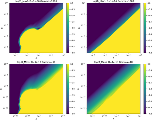
For the parameter study, the decimal logarithm of the maximum radius of the crystal R Max = X Max γ 2 $R_{\mathrm{Max}} = \sqrt {\frac{X_{\mathrm{Max}}}{\gamma ^2}}$ is plotted over A and B for different values for the parameters D ¯ $\bar{D}$ and γ. It can be seen in Figure 7 that in most cases, there is a clear cut between extremely large values, which are shown in yellow, and small values, which are shown in blue. Only in the bottom left corner of the left hand plots, so with large values for D ¯ $\bar{D}$ and small values for A, the transition becomes more blurry.
Details are in the caption following the image
Plots of parameter study with full range of color scaling.

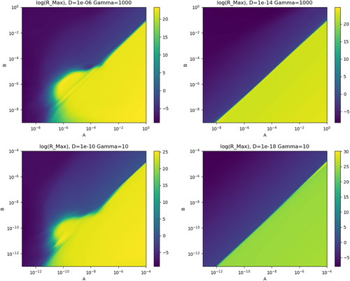
For better visibility, another set of plots is created in Figure 8 with an adjusted color scaling. In this case, crystals that have a maximum radius that is larger than 1 dm are shown in yellow, which means that those crystals are considered stable. Crystals with a maximum radius that is smaller than 1 mm are shown in blue. These crystals are considered unstable and would recrystallize. Values for the maximum radius that are between 1 dm and 1 mm are shown in green and show a transition area. In the right hand plots, the edge of the yellow area is a straight line in the double-logarithmic plot. When comparing the top-right plot with the bottom-right plot, it is striking that the transition area is a lot wider for small values of γ than for big values. On the other hand, the width of the transition is quite similar when comparing the bottom-left with the bottom-right plot. The left-hand plots do not have this shape. For values of A that are larger than 10 4 s 1 $10^{-4} \,\mathrm{s}^{-1}$ , the shape of the yellow area is similar to the other plots. For smaller values of A, the shape of the yellow area is different though. For small values of A (about 10 7 s 1 $10^{-7} \,\mathrm{s}^{-1}$ ), there is a steep gradient for the values of B where the transition takes place. For medium values of A, the gradient of the values of B becomes flatter and even decreases. This could mean that the parameter D ¯ $\bar{D}$ has a large influence on the shape of the transition area for values of A that are smaller than 10 4 s 1 $10^{-4} \,\mathrm{s}^{-1}$ .

Details are in the caption following the image
Plots of parameter study with adjusted range of color scaling.

5 CONCLUSION AND OUTLOOK

A model for the evolution of size, dislocation density, and magnesium concentration of an olivine crystal has been introduced and successfully implemented numerically. The parameter study has shown that the model has a high sensitivity to changes of the parameters A, B, and γ whilst changes to parameter D ¯ $\bar{D}$ only has a small effect when combined with large values of A, but has a significant influence when combined with small values of A. Generally, the model shows stark contrasts between extremely high and extremely low values for both the maximum radius of the crystals and the lifespan of them.

In the future, the causes for the extreme effect of D ¯ $\bar{D}$ in the parameter study should be investigated. Furthermore, our aim is to find a mathematical formulation for the threshold between large and small values of RMax as they correspond with the stability of the crystal.

ACKNOWLEDGMENTS

Open access funding enabled and organized by Projekt DEAL.

      The full text of this article hosted at iucr.org is unavailable due to technical difficulties.