Volume 23, Issue 4 e202300034
RESEARCH ARTICLE
Open Access

Relaxation approach for optimization of free boundary problems

Corinna Zurloh

Corresponding Author

Corinna Zurloh

Rheinland-Pfälzische Technische Universität Kaiserslautern-Landau, Kaiserslautern, Germany

Correspondence

Corinna Zurloh, Rheinland-Pfälzische Technische Universität Kaiserslautern-Landau, Gottlieb-Daimler-Str. 48, 67663 Kaiserslautern, Germany.

Email: [email protected]

Search for more papers by this author
René Pinnau

René Pinnau

Rheinland-Pfälzische Technische Universität Kaiserslautern-Landau, Kaiserslautern, Germany

Search for more papers by this author
First published: 21 November 2023

Abstract

We consider an optimal control problem (OCP) constrained by a free boundary problem (FBP). FBPs have various applications such as in fluid dynamics, flow in porous media or finance. For this work we study a model FBP given by a Poisson equation in the bulk and a Young-Laplace equation accounting for surface tension on the free boundary. Transforming this coupled system to a reference domain allows to avoid dealing with shape derivatives. However, this results in highly nonlinear partial differential equation (PDE) coefficients, which makes the OCP rather difficult to handle. Therefore, we present a new relaxation approach by introducing the free boundary as a new control variable, which transforms the original problem into a sequence of simpler optimization problems without free boundary. In this paper, we formally derive the adjoint systems and show numerically that a solution of the original problem can be indeed asymptotically approximated in this way.

1 INTRODUCTION

Free boundary problems (FBPs) occur in various fields of application. These include, for example, solidification, technical textiles, or thin film manufacturing processes [1-3]. Phase separation and optimal control problems (OCPs) constrained by the Stefan problem have been widely studied [2, 4-6]. Many of these problems have in common that there is a relation between the surface tension and the curvature of the boundary [7, 8].

In this paper, we study a model FBP that is very similar to the one considered by Saavedra and Scott [9]. Analytical results such as existence and uniqueness of solutions, existence of a minimizer and first and second order optimality conditions are shown by Antil et al. [10, 11]. Throughout this work we assume that the free boundary Γ γ $\Gamma _\gamma$ (dashed line) is represented as a graph of a function γ, cf. Figure 1 . The model consists of two equations: a Poisson equation, which describes the quantity in the interior of the domain, and a Young-Laplace equation, which connects the surface tension to the curvature of the free boundary.
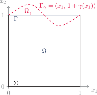
Details are in the caption following the image
Ω γ $\Omega _{\gamma }$ is the physical domain of the original FBP with boundary Ω γ = Σ Γ γ $\partial \Omega _{\gamma }=\Sigma \cup \Gamma _{\gamma }$ . The fixed part of the boundary is denoted by Σ and Γ γ $\Gamma _{\gamma }$ is free. We assume that the top boundary is given in graph form through γ. By transforming the domain Ω γ $\Omega _\gamma$ onto a reference domain Ω, we obtain a fixed top boundary Γ. The complete boundary of Ω is given by Ω = Γ Σ $\partial \Omega =\Gamma \cup \Sigma$ . All analysis and computations are done on Ω.

Free boundaries make the optimization highly complex and costly, particularly the derivation of the necessary optimality conditions and efficient numerical handling. When solving OCPs with FBPs, besides the state variables, the domain is also an unknown. To avoid having to deal with shape derivatives, we transform the FBP to a fixed domain. This is done at the expense of highly nonlinear PDE coefficients.

In this paper, we propose a relaxation-based approach that allows solving a sequence of simpler optimization problems instead of the optimization problem with the coupled constraint. Thereby we use the free boundary as a control, which is an idea already presented by Volkov [3, 12, 13].

This paper is organized as follows. In the remainder of this section we formulate the model FBP on a reference domain so that we do not have to deal with shape derivatives. We also state the nonlinear PDE constrained OCP and the relaxed OCP. Section 2 is devoted to the analysis of the well-posedness of the relaxed OCP and the formal derivation of the adjoint systems. The numerical solution of the OCPs based on a Broyden-Fletcher-Goldfarb-Shanno (BFGS) method is covered in Section 3. Here, we also show that the sequence of minimizers converges towards a minimizer of the original optimization problem as desired. We conclude in Section 4 with a summary and outlook.

1.1 Coupled state problem

We consider a model FBP on a domain Ω γ R 2 $\Omega _{\gamma }\subset \mathbb {R}^2$ similar to the problem analyzed by Antil et al. [10]. The difference is that we do distributed control, whereas their control variable u acts on the boundary. The top boundary Γ γ $\Gamma _\gamma$ of the physical domain Ω γ $\Omega _\gamma$ is free and parametrized by γ, compare Figure 1. Throughout this work we require that γ is Lipschitz continuous with constant 1, that is, | d x 1 γ | 1 a.e. I = ( 0 , 1 ) $|\textrm {d}_{x_1}\gamma |\le 1 \text{ a.e. } I=(0,1)$ , which ensures that | γ | 1 / 2 $|\gamma |\le 1/2$ . The governing equations are given by a Poisson equation in the bulk and a Young-Laplace equation accounting for surface tension on the free boundary. In order not to deal with changes in the domain when we consider OCPs for the FBP, we transform Ω γ $\Omega _\gamma$ to Ω = ( 0 , 1 ) 2 $\Omega =(0,1)^2$ and Γ γ $\Gamma _\gamma$ to Γ = ( 0 , 1 ) × { 1 } $\Gamma = (0,1)\times \lbrace 1\rbrace$ , compare with ref.[10]. Consequently, the coefficients in our PDE are highly nonlinear. Further, we identify the function spaces on Γ and I = ( 0 , 1 ) $I=(0,1)$ . Since we are only interested in small perturbations of the flat case γ = 0 $\gamma =0$ , we assume like in ref. [10] that the curvature can be linearized and our control is scaled accordingly.

This results in the following transformed PDE problem
div ( A [ γ ] y ) = u in Ω , $$\begin{equation} -{\textrm {div}}({A[\gamma ]}\nabla y) \eqcellsep = \eqcellsep u\qquad \text{ in }{\Omega },\eqbreak \end{equation}$$ (1a)
y = 0 on Ω , $$\begin{equation} y \eqcellsep = \eqcellsep 0\qquad \text{ on }{\partial \Omega },\eqbreak \end{equation}$$ (1b)
κ d x 1 2 γ + A [ γ ] y · ν = 0 on I , $$\begin{equation} -\kappa {\textrm {d}_{x_1}^2}\gamma + {A[\gamma ]\nabla }y \cdot {\nu } \eqcellsep = \eqcellsep 0\qquad \text{ on } {I},\eqbreak \end{equation}$$ (1c)
γ ( 0 ) = γ ( 1 ) = 0 , $$\begin{equation} \gamma (0) = \gamma (1) \eqcellsep = \eqcellsep 0, \end{equation}$$ (1d)
where κ > 0 $\kappa >0$ is some fixed constant, ν is the outward pointing unit normal vector along Ω $\partial \Omega$ and A is the Nemytskii operator defined by
A [ γ ] = 1 + γ ( x 1 ) d x 1 γ ( x 1 ) x 2 d x 1 γ ( x 1 ) x 2 1 + ( d x 1 γ ( x 1 ) x 2 ) 2 1 + γ ( x 1 ) . $$\begin{equation*} A[\gamma ] = \def\eqcellsep{&}\begin{bmatrix} 1+\gamma (x_1) & -\mathrm{d}_{x_1}\gamma (x_1)x_2 \\[10pt] -\mathrm{d}_{x_1}\gamma (x_1)x_2 & \dfrac{1+(\mathrm{d}_{x_1}\gamma (x_1)x_2)^2}{1+\gamma (x_1)} \end{bmatrix}. \end{equation*}$$

1.2 Optimal control problems

We want to optimize in a Hilbert space setting, so we consider the following spaces. Let U = L 2 ( Ω ) $U=L^2(\Omega )$ , Y = H 2 ( Ω ) H 0 1 ( Ω ) $Y = H^2(\Omega )\cap H_0^1(\Omega )$ and G = H 3 ( I ) H 0 1 ( I ) $G = H^3(I)\cap H_0^1(I)$ . The reason for those high regularities is discussed later.

Graph as state variable

Our goal is to find an optimal control u U a d U $u\in U_{ad}\subseteq U$ in the set of admissible controls, so that the solution pair ( y , γ ) Y × G $(y, \gamma )\in Y\times G$ of the FBP approximates a given boundary γ d : I R $\gamma _d: I\rightarrow \mathbb {R}$ and potential y d : Ω R $y_d: \Omega \rightarrow \mathbb {R}$ . Hence, we consider the following tracking-type cost functional
J 0 ( y , γ , u ) : = λ γ 2 γ γ d H 3 ( I ) 2 + λ y 2 ( y y d ) 1 + γ L 2 ( Ω ) 2 + λ u 2 u L 2 ( Ω ) 2 $$\begin{equation} J_0(y, \gamma ,u):= \frac{\lambda _{\gamma }}{2} \Vert \gamma -\gamma _d\Vert ^2_{H^3(I)}+\frac{\lambda _y}{2} \Vert (y-y_d)\sqrt {1+\gamma }\Vert ^2_{L^2({\Omega })} + \frac{\lambda _u}{2} \Vert u\Vert ^2_{L^2({\Omega })} \end{equation}$$ (2)
for fixed parameters λ γ , λ y , λ u 0 $\lambda _\gamma , \lambda _y,\lambda _u\ge 0$ weighting the objective and the control costs, respectively. Note, that 1 + γ $\sqrt {1+\gamma }$ is the square root of the functional determinant of the transformation of Ω γ $\Omega _\gamma$ to Ω. Treating the graph as a state variable the minimization problem reads
min u U a d J 0 ( y , γ , u ) , s. t. ( y , γ ) Y × G solves (1) in H 1 ( Ω ) × H 1 ( I ) , | d x 1 γ | 1 , a.e. in I , $$\begin{equation} \begin{split} \min _{u\in U_{ad}} \,&J_0(y,\gamma ,u),\\[-3pt] \text{s.\,t. } & (y,\gamma )\in Y\times G \text{ solves (1) in } H^{-1}(\Omega )\times H^{-1}(I), \\[-3pt] & |\mathrm{d}_{x_1}\gamma |\le 1, \quad \text{a.e. in } I, \end{split} \end{equation}$$ (P0)
where U a d $U_{ad}$ is a set of admissible controls.

Graph as control variable

The PDE constraint in (P0) is a highly nonlinear and numerically challenging due to the coupling with the free boundary. To simplify the problem we incorporate the Equation (1c) for γ into the cost function; see also refs.[3, 12]. By this relaxation the graph becomes an extra control variable. We introduce a parameter λ > 0 $\lambda >0$ , relax the residual of the equation for γ on the top boundary Γ and solve the resulting minimization problem. The relaxation is done in an L2-sense, which yields
min ( γ , u ) G a d × U a d J λ ( y , γ , u ) : = J 0 ( y , γ , u ) + λ 2 κ d x 1 2 γ + A [ γ ] y · ν L 2 ( Γ ) 2 s. t. y Y solves (1a)-(1b) in H 1 ( Ω ) $$\begin{equation} \begin{split} \min _{(\gamma , u)\in G_{ad}\times U_{ad}} \,&J_\lambda (y, \gamma ,u):= J_0(y,\gamma , u)\, + \frac{\lambda }{2} \Vert -\kappa \mathrm{d}_{x_1}^2\gamma +A[\gamma ]\nabla y\cdot \nu \Vert ^2_{L^2(\Gamma )} \\ \text{s.\,t. } & y\in Y \text{ solves (1a)-(1b) in } H^{-1}(\Omega ) \end{split} \end{equation}$$ ( P λ ${{P_\lambda }}$ )
with state variable y and control variables γ and u. Here, G and U are the function spaces from above with suitable admissible subsets G a d $G_{ad}$ and U a d $U_{ad}$ specified later. Note, that the state constraint in (P0) becomes a control constraint, which is contained in G a d $G_{ad}$ .

2 ANALYSIS

In the following we assume
  • (A1) the set of admissible controls U a d $U_{ad}$ or G a d × U a d $G_{ad}\times U_{ad}$ , respectively, is a weakly closed and convex subset of the control space,
  • (A2) the desired potential y d $y_d$ is in L 2 ( Ω ) $L^2(\Omega )$ , and the desired boundary γ d $\gamma _d$ in H 3 ( I ) H 0 1 ( I ) $H^3(I)\cap H_0^1(I)$ .
It is, for example, reasonable to consider the unconstrained case U a d = U $U_{ad}=U$ and a small ball around γ = 0 $\gamma =0$ for G a d G $G_{ad}\subseteq G$ . This choice of G a d $G_{ad}$ is consistent with the small perturbations assumption and linearization of the curvature in (1c).

2.1 Well-posedness of ( P λ $P_\lambda$ )

Due to the highly nonlinear coefficients in the PDE constraint of ( P λ $P_\lambda$ ), the following theorem provides the necessary existence and uniqueness of a solution y.

Theorem 2.1. (Existence and Uniqueness of forward problem)For all γ G $\gamma \in G$ with | d x 1 γ | 1 $|\mathrm{d}_{x_1}\gamma |\le 1$ and right-hand sides u U $u\in U$ the PDE (1a)–(1b) has a unique solution y H 2 ( Ω ) H 0 1 ( Ω ) $y\in H^2(\Omega )\cap H_0^1(\Omega )$ .

Proof.The PDE (1a)–(1b) is uniformly elliptic, since A [ γ ] $A[\gamma ]$ is positive definite; compare ref. [9]. Clearly, Ω = ( 0 , 1 ) 2 $\Omega =(0,1)^2$ is a convex, bounded, and open subset of R 2 $\mathbb {R}^2$ and the right-hand side of the PDE is in L 2 ( Ω ) $L^2(\Omega )$ by assumption. By Sobolev's embedding theorem [14, Thm. 5.4], we have

H 2 ( I ) C 1 , 1 / 2 ( I ¯ ) C 0 , 1 ( I ¯ ) $$\begin{equation*} H^2(I)\hookrightarrow C^{1,1/2}(\bar{I}) \hookrightarrow C^{0,1}(\bar{I}) \end{equation*}$$
for bounded I R $I\subset \mathbb {R}$ . Since we require γ H 3 ( I ) $\gamma \in H^3(I)$ , we observe γ , d x 1 γ C 0 , 1 ( I ¯ ) $\gamma , \mathrm{d}_{x_1}\gamma \in C^{0,1}(\bar{I})$ , and all together we can conclude that A [ γ ] ( C 0 , 1 ( Ω ¯ ) ) 2 × 2 $A[\gamma ] \in (C^{0,1}(\bar{\Omega }))^{2\times 2}$ . By [15, Thm. 3.2.1.2] we get the existence and uniqueness of a solution y H 2 ( Ω ) H 0 1 ( Ω ) $y\in H^2(\Omega )\cap H_0^1(\Omega )$ to (1a)–(1b). $\Box$

Remark 2.2.The high regularity of γ implies y H 2 ( Ω ) $y\in H^2(\Omega )$ . Hence, the co-normal derivative A [ γ ] y · ν $A[\gamma ] \nabla y\cdot \nu$ along the boundary Γ is well-defined in L 2 ( I ) L 2 ( Γ ) $L^2(I)\cong L^2(\Gamma )$ ; see, for example [16].

To show the existence of an optimal control for any fixed λ > 0 $\lambda >0$ we collect some properties of the state Equation (1a)–(1b) in weak form. We define the state operator ( y , ( γ , u ) ) Y × ( G × U ) e ( y , γ , u ) Y $(y,(\gamma , u))\in Y \times (G\times U) \mapsto e(y,\gamma , u)\in Y^*$ , where Y $Y^*$ denotes the dual space of Y and · , · Y , Y $\langle \cdot , \cdot \rangle _{Y^*,Y}$ the corresponding dual pairing, by
e ( y , γ , u ) , h Y , Y : = Ω ( A [ γ ] y h + u h ) d x . $$\begin{equation*} \langle e(y,\gamma ,u), h\rangle _{{Y}^*, Y}:= \int _\Omega ({A[\gamma ]}\nabla y\nabla h + uh)\mathrm{d}x. \end{equation*}$$
The solution operator σ : G × U Y $\sigma : {G\times U}\rightarrow {Y}$ with σ ( γ , u ) = y for all ( γ , u ) G a d × U a d $\sigma (\gamma , u)=y\, \text{ for all } (\gamma , u)\in G_{ad}\times U_{ad}$ maps a given control ( γ , u ) G a d × U a d $(\gamma , u)\in {G}_{ad}\times U_{ad}$ to its unique solution y Y $y\in {Y}$ by Theorem 2.1. It is easy to see by standard arguments, that e gives rise to a continuous and H1-coercive bilinear form. It is further weakly continuous, which can be shown by using the compact embedding H 3 ( I ) C 1 ( I ) $H^3(I)\hookrightarrow C^1(I)$ , which guarantees pointwise convergence of A [ γ k ] A [ γ ] $A[\gamma _k]\rightarrow A[\gamma ]$ for some sequence ( γ k ) k G $(\gamma _k)_k\in G$ .

Theorem 2.3. (Existence of Minimizer)Let λ > 0 $\lambda >0$ be fixed and assumptions (A1) and (A2) hold. Assume further that ( 0 , 0 ) G a d × U a d $(0,0)\in G_{ad}\times U_{ad}$ . With these assumptions there exists ( γ , u ) G a d × U a d $(\gamma ^*,u^*)\in G_{ad}\times U_{ad}$ such that

( γ , u ) = a r g m i n ( γ , u ) G a d × U a d J λ ( γ , u ) , $$\begin{equation*} (\gamma ^*, u^*)=\underset{(\gamma , u)\in {G}_{ad}\times U_{ad}}{\textup {argmin}}\,\tilde{J}_{\lambda }(\gamma , u), \end{equation*}$$
where J λ ( γ , u ) : = J λ ( σ ( γ , u ) , γ , u ) $\tilde{J}_\lambda (\gamma , u) := J_\lambda (\sigma (\gamma , u), \gamma , u)$ denotes the reduced cost functional.

The proof follows standard arguments; see, for example [17].

2.2 Formal Lagrange principle

Due to limited space, we only present the formal adjoint equations to (P0) and ( P λ $P_\lambda$ ). Assuming enough regularity to ensure Fréchet differentiability, we apply the Lagrangian multiplier technique, where r denotes the Lagrange multiplier for the equation constraint and s is the corresponding one for the additional boundary condition; see, for example [18] or [17].

The adjoint equations to (P0) in strong form can be derived analogously as in ref. [10], where also the definition of A 1 [ γ ] $A_1[\gamma ]$ and A 2 [ γ ] $A_2[\gamma ]$ can be found. They read
div ( A [ γ ] r ) = λ y ( y y d ) ( 1 + γ ) in Ω , $$\begin{equation} -{\textrm {div}}({A[\gamma ]}\nabla r) \eqcellsep = \eqcellsep \lambda _y(y-y_d)({1+\gamma }) \qquad \text{ in }{\Omega },\eqbreak \end{equation}$$ (3a)
r = s on Γ , $$\begin{equation} r \eqcellsep = \eqcellsep s\qquad\hspace*{68pt} \text{ on }{\Gamma },\eqbreak \end{equation}$$ (3b)
r = 0 on Σ , $$\begin{equation} r \eqcellsep = \eqcellsep 0\qquad\hspace*{68pt} \text{ on }\Sigma , \end{equation}$$ (3c)
and
κ d x 1 2 s = λ γ ( γ γ d ) λ γ ( d x 1 2 γ d x 1 2 γ d ) + λ γ ( d x 1 4 γ d x 1 4 γ d ) λ γ ( d x 1 6 γ d x 1 6 γ d ) + λ y 2 0 1 | y y d | 2 d x 2 0 1 A 1 [ γ ] y · r d x 2 + d x 1 0 1 A 2 [ γ ] y · r d x 2 on I , $$\begin{align} -{\kappa }\mathrm{d}_{x_1}^2s=&\,\lambda _{\gamma }(\gamma -\gamma _d) - \lambda _{\gamma }(\mathrm{d}_{x_1}^2\gamma -\mathrm{d}_{x_1}^2\gamma _d) + \lambda _{\gamma }(\mathrm{d}_{x_1}^4\gamma -\mathrm{d}_{x_1}^4\gamma _d) - \lambda _{\gamma }(\mathrm{d}_{x_1}^6\gamma -\mathrm{d}_{x_1}^6\gamma _d) && \nonumber \\ & +\frac{\lambda _y}{2} \int _0^1|y-y_d|^2\mathrm{d}{x_2} -\int _0^1 A_1[\gamma ]\nabla y\cdot \nabla r\,\mathrm{d}x_2 + \mathrm{d}_{x_1}{\left(\int _0^1 A_2[\gamma ]\nabla y\cdot \nabla r\,\mathrm{d}{x_2}\right)}&&\text{ on }{I}, \end{align}$$ (3d)
s ( 0 ) = s ( 1 ) = 0 . $$\begin{align} s(0) = &\,s(1) = 0.&& \end{align}$$ (3e)
The optimality condition of the Lagrange function L0 for problem (P0) is simply u L 0 ( u ) = ( λ u u + r ) $\nabla _u L_0(u) = -(\lambda _uu+r)$ .
The adjoint equation to ( P λ $P_\lambda$ ) is
div ( A [ γ ] r ) = λ y ( y y d ) ( 1 + γ ) in Ω , $$\begin{equation} -{\textrm {div}}({A[\gamma ]}\nabla r) \eqcellsep = \eqcellsep \lambda _y(y-y_d)({1+\gamma }) \qquad\hspace*{28pt} \text{ in }{\Omega },\eqbreak \end{equation}$$ (4a)
r = λ ( κ d x 1 2 γ A [ γ ] y · ν ) on Γ , $$\begin{equation} r \eqcellsep = \eqcellsep -\lambda (\kappa {\mathrm{d}_{x_1}^2}\gamma -{A[\gamma ]\nabla } y\cdot {\nu })\qquad \text{ on }{\Gamma },\eqbreak \end{equation}$$ (4b)
r = 0 on Σ , $$\begin{equation} r \eqcellsep = \eqcellsep 0\qquad\hspace*{94pt} \text{ on }\Sigma , \end{equation}$$ (4c)
with only one adjoint variable r to y.
Denoting the corresponding Lagrange function with L γ $L_\gamma$ the variational equation for γ is computed via
D γ L λ , γ G , G = 0 1 ( a d x 1 3 γ + b d x 1 2 γ + c d x 1 γ + d γ ) d σ $$\begin{align} \langle D_\gamma L_\lambda , \gamma \rangle _{G^{*}, G} = \int _0^1(a\mathrm{d}_{x_1}^3\gamma + b\mathrm{d}_{x_1}^2\gamma +c\mathrm{d}_{x_1}\gamma +d\gamma )\,\mathrm{d} \sigma \end{align}$$ (5a)
with
d = λ γ ( γ γ d ) + λ y 2 0 1 ( y y d ) 2 d x 2 + λ ( κ d x 1 2 + A [ γ ] y · ν ) A 1 [ γ ] y · ν + A 1 [ γ ] y · ν r 0 1 A 1 [ γ ] y · r d x 2 , c = λ γ ( d x 1 γ d x 1 γ d ) + λ ( κ d x 1 2 + A [ γ ] y · ν ) A 2 [ γ ] y · ν + A 2 [ γ ] y · ν r 0 1 A 2 [ γ ] y · r d x 2 , b = λ γ ( d x 1 2 γ d x 1 2 γ d ) + λ ( κ d x 1 2 + A [ γ ] y · ν ) ( κ ) , and a = λ γ ( d x 1 3 γ d x 1 3 γ d ) . $$\begin{align} \begin{aligned} d =&\, \lambda _\gamma (\gamma -\gamma _d) + \frac{\lambda _y}{2} \int _0^1(y-y_d)^2\,\mathrm{d}x_2+ \lambda (-\kappa \mathrm{d}_{x_1}^2+A[\gamma ]\nabla y\cdot \nu )A_1[\gamma ]\nabla y\cdot \nu \\ & + A_1[\gamma ]\nabla y\cdot \nu r-\int _0^1 A_1[\gamma ]\nabla y\cdot \nabla r\mathrm{d}x_2 ,\\ c =&\, \lambda _\gamma (\mathrm{d}_{x_1}\gamma -\mathrm{d}_{x_1}\gamma _d) + \lambda (-\kappa \mathrm{d}_{x_1}^2+A[\gamma ]\nabla y\cdot \nu )A_2[\gamma ]\nabla y\cdot \nu \\ & + A_2[\gamma ]\nabla y\cdot \nu r-\int _0^1 A_2[\gamma ]\nabla y\cdot \nabla r\mathrm{d}x_2, \\ b =&\, \lambda _\gamma (\mathrm{d}_{x_1}^2\gamma -\mathrm{d}_{x_1}^2\gamma _d) + \lambda (-\kappa \mathrm{d}_{x_1}^2+A[\gamma ]\nabla y\cdot \nu )(-\kappa ), \text{ and}\\ a =&\, \lambda _\gamma (\mathrm{d}_{x_1}^3\gamma -\mathrm{d}_{x_1}^3\gamma _d). \end{aligned} \end{align}$$ (5b)
Consequently, to identify the descent direction, we need to compute an H 3 ( I ) $H^3(I)$ -representative g of the derivative by solving the weak form of a 6 t h $6th$ order equation. The optimality condition of the Lagrange function L λ $L_\lambda$ of ( P λ $P_\lambda$ ) with respect to u is as before, so the complete one is given by
( γ , u ) L λ ( γ , u ) = g ( λ u u + r ) . $$\begin{equation*} \nabla _{(\gamma ,u)} L_\lambda (\gamma , u) = \def\eqcellsep{&}\begin{pmatrix} g \\ -(\lambda _u u +r) \end{pmatrix}. \end{equation*}$$

3 NUMERICAL SOLUTION OF THE OCPs

Setting

To solve the optimization problems (P0) and ( P λ $P_\lambda$ ) numerically, we use the BFGS algorithm together with the Armijo rule [18]. We choose γ d $\gamma _d$ and y d $y_d$ as the solution pair of (1) for
u ( x 1 , x 2 ) = f 2 π σ 2 exp s 4 σ 2 [ ( x 1 μ ) 2 + ( x 2 μ ) 2 ] $$\begin{equation*} u(x_1,x_2)=\frac{f}{2\pi \sigma ^2}\exp {{\left(-\frac{s}{4\sigma ^2}[(x_1-\mu )^2 + (x_2-\mu )^2]\right)}} \end{equation*}$$
inspired by a two-dimensional scaled density of the normal distribution with μ = 0.5 , σ = 1 , f = 150 $\mu =0.5, \, \sigma =1,\, f=150$ , and s = 20 $s=20$ . The derivative in x2 direction of this function u is quite large, which causes an actual deformation of the top boundary and gives an interesting optimization setting. It further ensures that γ d $\gamma _d$ and y d $y_d$ are reachable. In the following the surface tension coefficient is fixed to κ = 1 $\kappa =1$ . Recall that the cost function consists of two tracking type terms for y d $y_d$ and γ d $\gamma _d$ and a regularization term for u. To get enough regularity of γ in the analysis we needed that the term γ γ d $\gamma -\gamma _d$ is measured in the H 3 ( I ) $H^3(I)$ -norm. However, for the numerical analysis we reduce these regularity assumptions and measure the difference only in L 2 ( I ) $L^2(I)$ . Since the case, where γ acts as a state variable, automatically yields a solution with H2-regularity, we want to ensure the same for the case where γ acts as a control variable. This is realized by computing suitable gradients and details are given below in (6). The parameters in the cost functional (2) are chosen as λ y = 1.0 , λ γ = 100 $\lambda _y = 1.0, \, \lambda _\gamma =100$ and λ u = 10 2 $\lambda _u=10^{-2}$ . In the relaxed problem ( P λ $P_\lambda$ ) we initially choose λ = 10 2 $\lambda =10^{-2}$ . The asymptotic solution for λ $\lambda \rightarrow \infty$ is computed via a homotopy approach. In our implementation λ is increased by a fixed factor f λ = 10 $f_\lambda =10$ , until the residual of the equation J1 in the cost function of ( P λ $P_\lambda$ ) is smaller than a given tolerance chosen as t o l λ = 10 6 $tol_{\lambda }=10^{-6}$ . The critical point found for the maximal λ is compared to the critical point computed by (P0).

The PDE constraints are solved with a finite element method (FEM)in the framework of FENICS [19, 20]. For this purpose, the function spaces Y and U are discretized with continuous galerkin (CG) elements of first order. The function space G is discretized with CG elements of second order [20].

The optimization procedure is initialized with u = 0 $u=0$ and γ = 0 $\gamma =0$ and stopped when the termination criterion is fulfilled, which is composed of two conditions. Either the relative gradient norm is smaller than a given tolerance, or the relative change of the controls is no longer large. This second criterion has been shown to be reasonable by numerical experiments. The tolerances for both criteria are chosen as t o l = 10 3 $tol=10^{-3}$ .

Due to the discretization of G with second order CG elements, we have to be careful when implementing the H2–scalar product. To compute a gradient representant in H 2 ( I ) $H^2(I)$ numerically we need to solve the following equation
g , h H 2 ( I ) , n u m = 0 1 ( a d x 1 2 h + b d x 1 h + c h ) d x 1 $$\begin{align} \langle g, h\rangle _{H^2(I), num} = \int _0^1(a\mathrm{d}_{x_1}^2h+b\mathrm{d}_{x_1}h+ch)\,\mathrm{d}x_1 \end{align}$$ (6a)
with a , b , c $a,b,c$ as before. The notation · , · H 2 ( I ) , n u m $\langle \cdot ,\cdot \rangle _{H^2(I), num}$ denotes the numerical implementation of the H2–scalar product. Since we deal with CG elements, the derivative is a piecewise linear function by convention with possible discontinuities. Therefore we have to implement terms that give a continuous solution without any jumps at the interface of two elements. This is done with a Nitsche approach, for which we need the following two notations. Let v be a piecewise continuous function on a mesh T $\mathcal {T}$ . On a face F between two cells T1 and T2, we define the average operator and the jump operator as
{ v ( x ) } = 1 2 ( v 1 ( x ) + v 2 ( x ) ) and [ v ] = ( v 1 v 2 ) n 1 2 = ( v 2 v 1 ) n 2 2 $$\begin{equation*} \lbrace v(x)\rbrace =\frac{1}{2} (v_1(x)+v_2(x)) \quad \text{and} \quad [v]=\frac{(v_1-v_2)n_1}{2}=\frac{(v_2-v_1)n_2}{2} \end{equation*}$$
respectively, where n i $n_i$ are the outer normal vectors of the two cells. The numerical implementation of the H2–scalar product then reads
g , h H 2 ( I ) , n u m = 0 1 ( d x 1 2 g d x 1 2 h + d x 1 g d x 1 h + g h ) d x 1 η · { d x 1 2 w } [ d x 1 h ] d S i η · [ d x 1 2 w ] { d x 1 h } d S i η α h a v g [ d x 1 w ] [ d x 1 h ] d S i , $$\begin{align} \begin{aligned} \langle g,h\rangle _{H^2(I), num} =& \int _0^1 (\mathrm{d}_{x_1}^2g\mathrm{d}_{x_1}^2h+ \mathrm{d}_{x_1}g\mathrm{d}_{x_1}h+ gh)\, \mathrm{d}x_1 \\ &- \eta \cdot \int \lbrace \mathrm{d}_{x_1}^2w\rbrace [\mathrm{d}_{x_1}h] \mathrm{d}S_i - \eta \cdot \int [\mathrm{d}_{x_1}^2w] \lbrace \mathrm{d}_{x_1}h\rbrace \mathrm{d}S_i - \frac{\eta \alpha }{h_{avg}}\int [\mathrm{d}_{x_1}w][\mathrm{d}_{x_1}h] \mathrm{d}S_i, \end{aligned} \end{align}$$ (6b)
where the differential d S i $\mathrm{d}S_i$ denotes the integral along the inner boundaries of all elements. More details can be found in ref.[21].

Results

Repeatedly solving problem ( P λ $P_\lambda$ ) for increasing values of λ eventually leads to a critical point, where the second equation of the coupled PDE problem (1) is also satisfied in the weak sense. The evolution of the cost functional can be seen in Figure 2. The jumps result from the term λ J 1 $\lambda J_1$ in the cost function and enlarging λ. Between two jumps we see the evolution of the cost functional while computing a critical point of ( P λ $P_\lambda$ ) for fixed λ. Next to the composite cost functional, one sees the decrease in the term J1, which essentially measures the square of the residual of the second equation of the coupled PDE. The relation between the increase in λ and the decrease in J1 is somewhat better than linear, what we would expect. Note, however, that in ref.[22] it is shown for a different problem that the order of convergence can be better for solutions with higher regularity, which we might observe here as well. In our setting λ was increased from 10−2 to 103.

Details are in the caption following the image
Optimization results of control problem. (A) Cost functional with increased λ at jumps. (B) Corresponding mismatch J1 after each outer iteration with fixed λ.

It remains to illustrate that the final minimizer of ( P λ $P_\lambda$ ) converges towards the minimizer (P0) for finer discretizations. For this purpose, the difference of the minimizers are calculated for y , u $y, u$ and γ and plotted against the parameter λ for different grid sizes in Figure 3.

Details are in the caption following the image
Relative difference between critical point of state problem and critical points for y , u $y, u$ and γ as λ increases in regularized case.

In Figure 4 different (interim) solutions for γ are shown, including the final critical point of ( P λ $P_\lambda$ ), and various intermediate solutions for γ from 10−2 to 103. Next to it a zoom into the interesting part at the center of the interval is given. In both figures the critical point of (P0) is shown as well.

Details are in the caption following the image
Asymptotic behavior of γ for h = 1 64 $h=\frac{1}{64}$ . (A) Evolution of critical points of ( P λ $P_\lambda$ ) for λ from 10−2 to 103 with critical point γ $\gamma ^*$ of problem (P0). (B) Zoom into left figure.

4 CONCLUSION

We presented a highly nonlinear optimization problem for a FBP model that was transformed onto a reference domain and used a penalty method to relax the condition for the free boundary. First, the free boundary was treated as a state variable, while in the second approach it acts as a control variable. We stated results concerning the existence and uniqueness of solutions with H 2 ( Ω ) $H^2(\Omega )$ regularity to the state equation in the relaxed case. Further, we discussed the well-posedness of the OCP for the relaxed problem, which required a careful regularity analysis of the co-normal derivative involving the highly nonlinear Nemytskii operator A [ γ ] $A[\gamma ]$ . For numerical simulations, we formally calculated derivatives using the Lagrangian approach. Finally, we examined numerically the asymptotic behavior of the two OCPs for a reachable setting, underlining the feasibility of our approach.

ACKNOWLEDGMENTS

Open access funding enabled and organized by Projekt DEAL.

      The full text of this article hosted at iucr.org is unavailable due to technical difficulties.