
The Earth is nearly flat: Precise and approximate algorithms for detecting vulnerable regions of networks in the plane and on the sphere
Abstract
Several recent works shed light on the vulnerability of networks against regional failures, which are failures of multiple pieces of equipment in a geographical region as a result of a natural disaster. To enhance the preparedness of a given network to natural disasters, regional failures and associated Shared Risk Link Groups (SRLGs) should be first identified. For simplicity, most of the previous works assume the network is embedded on a Euclidean plane. Nevertheless, they are on the Earth's surface; this assumption causes distortion. In this work, we generalize some of the related results on the plane to the sphere. In particular, we focus on algorithms for listing SRLGs as a result of regional failures of circular or other fixed shape.
Abbreviations
-
- PSRLG
-
- Probabilistic SRLG
-
- SRLG
-
- Shared Risk Link Group
1 INTRODUCTION
Serious network outages are happening with increasing frequency due to disasters (such as earthquakes, hurricanes, tsunamis, tornadoes, etc.) that take down almost every equipment in a geographical area (see 9 for a recent survey conducted within COST Action RECODIS 21 on strategies to protect networks against large-scale natural disasters). Such failures are called regional failures and can have many locations, shapes, and sizes.
Due to the huge importance of telecommunication services, improving the preparedness of networks to regional failures is becoming a key issue 6, 8, 10-12, 16, 17, 19, 24. Roughly speaking, protecting networks against regional failures is dealt with either by using geometric tools 1, 7, 19, 25-27, 29 or by reducing massively the problem space to a set candidate locations of failures 6, 10, 11, 16, 17, 24. Nevertheless, both approaches require a detailed knowledge of the geometry of the network topology, such as the precise GPS coordinates of nodes and cable conduits' routes, and the statistics of past disasters.
In many works, regional failures are computed by transforming the geographical coordinates of an existing network into a plane, which introduces distortion. Depending both on the geographical area of the network and on the transforming procedure, this distortion can vary from negligible to significant. For example, the backbone network of a small-to-medium size country is not suffering a significant distortion when compared with the uncertainty of the available geographical data, but when turning to networks covering a large country, a continent, or even multiple continents, there is no projection which can hide the spherical-like geometry of the Earth's surface (see Figure 1 taken from 23). For example, while the territory of continental US can be mapped onto a plane with 4% distortion 23, if we want to investigate bigger networks, clearly there is no projection which can hide the spherical-like geometry of the Earth.

There are reasons why one should analyze the global communication network as a whole: Electromagnetic storms induced by the Sun's coronal mass ejections could cause severe simultaneous failures of electric and communication networks all over the Earth1.
Backbone networks are designed to protect a given pre-defined list of failures, called Shared Risk Link Groups (SRLGs). Network recovery mechanisms are efficient if this SRLG list covers the most probable failure scenarios while having a manageable size.
An SRLG is called regional if it aims to characterize a failure damaging the network only in a bounded geographical area. It is still ongoing research on how to define and compute efficiently regional SRLG lists 25, 26, 29. A common simplification of these works is that they compute the list of SRLGs on a planar representation of the networks; thus, our focus is to generalize these approaches to the sphere.
An SRLG consists of a set of network links, while node failures are implicitly defined (a node is considered to be failed with the SRLG if all its adjacent edges are part of the SRLG). If a failure f is listed as an SRLG, it is a common approach to skip listing any subset of f (if the network is protected to f, it is also protected to any of its subsets) and, therefore, it is enough to list the maximal SRLGs caused by disasters.
Another issue is that the number of the listed SRLGs has to be kept low. With this aim, there is a common practice to fix the shape of the disasters 1, 27 with the assumption that every link intersecting the disaster area is destroyed, while the rest of the network is left intact. Among the possible geometric failure shapes, the most natural one is the circular disk, as it is compact, and is invariant to rotation. One possibility is to overestimate the possible failures with circular disks (or any other fixed geometric shape), which yields short SRLG lists. However, it is not clear what is the cost of this overestimation. In most of this work, we choose to overestimate the disasters by circular disks with a maximum size according to one among many possible measures, while we also briefly tackle overestimations with different geometric shapes.
- maximal r-range SRLG list: list of maximal link sets that can be hit by a disk with radius at most r.
- maximal k-node SRLG list: list of maximal link sets that can be hit by a disk hitting at most k nodes.
- maximal k-link SRLG list: list of maximal link sets that can be hit by a disk hitting at most k links.
To distinguish between lists obtained from planar and spherical representation, we will include attribute planar or spherical in the list names (e.g., maximal spherical r-range SRLG list) when needed for clarification.
It turns out that in all three mentioned cases, the size of the maximal SRLG list is linear in the network size in practice, and can be computed in low-polynomial time both in the planar case (maximal r-range list: 25, k-node: 29, k-link: 20) and the spherical case.
This paper is an extension of 30, which is, to the best of our knowledge, the first study on enumerating regional SRLG lists in a spherical model. Also, in 30, the first comparison of the spherical and planar representations was provided. It is shown through examples that precise polynomial algorithms could be designed for spherical representation of the networks. In our experience, these algorithms are only 2 times slower than their planar pairs. We also believe that using our approach, resilient routing and network design results 14 can be further enhanced. Compared to the conference version of our paper 30, we have (1) included Section 4.2 presenting approximate algorithms on enumerating the maximal failures induced by arbitrary disaster shapes, (2) provided an enhanced mathematical analysis of algorithms presented Sections 4.1 and 4.2, and (3) in Section 5 added simulation results showing that the difference between the planar and spherical representations of the network can result in different SRLG lists even in case of networks having a geographic extension as small as  .
.
As there are many mathematical derivations in the rest of the paper, we would like to summarize the concepts in plain text once again here for the sake of readability. As learned from previous studies, all of r-range, k-node, and l-link lists can be precisely calculated in low-polynomial time of the network size in case of planar representation of the network. Our first goal was to show that considering spherical embeddings of the networks the possibility of designing low-polynomial time algorithms for determining these SRLG lists remains. We demonstrated this phenomenon in Section 3 by designing an algorithm capable of determining the r-range SLRG list both in the planar and spherical case in low-polynomial time of the network elements. The existence of fast precise algorithms is good news, however, their drawback is that intuitively the faster they are, the harder they are to implement. This fact motivates our second goal, namely designing a framework of simple and fast algorithms capable of determining all the mentioned SRLG lists in both planar and spherical representation with enough precision, which are presented in Section 4.1. Our third and final goal is to show how simple approaches can be applied to more general models too: while in most of this study, we concentrated on disasters having a shape overestimated by a disk, Section 4.2 gives an outlook for designing easy-to-implement algorithms for essentially arbitrary disaster shapes.
The remaining of the paper is organized as follows. Section 2 describes the network representation model together with the assumptions made. In Section 3, we present an example of a polynomial algorithm for computing maximal SRLG lists, handling both the planar and spherical cases. While in Section 4.1, a faster and more flexible approximate approach is presented for solving the same problem, Section 4.2 gives an outlook for designing algorithms for arbitrary disaster shapes. Simulation results are presented in Section 5 and, finally, we draw the conclusions in Section 6.
2 MODEL AND ASSUMPTIONS
Throughout the paper, we will consider two types of embeddings of the network: embedding in Euclidean planar and spherical geometry.
The network is modeled as an undirected connected geometric graph  with n = | V | ≥ 3 nodes and m = | ℰ| edges stored in a lexicographically sorted list. The nodes of the graph are embedded as points in the Euclidean plane or sphere, and their precise coordinates are considered to be given in 2D and 3D Cartesian coordinate system in the planar and spherical cases, respectively. Note that if coordinates are given in polar system (in case of spherical geometry), one can easily transform them to Cartesian at the very beginning.
When speaking of planar geometry, for each edge e, there is a polygonal chain (or simply polyline) el in the plane in which the edge lies (see Figure 2). Parameter γ will be used to indicate the maximum number of line segments a polyline el can have. Naturally, in spherical case, the polyline of an edge refers to a series of geodesics. Note that this model covers special cases when edges are considered as line segments (geodesics).

 with polylines, n = 17, γ = 4
It will be assumed that basic arithmetic functions ( ) have constant computational complexity. For simplicity, we assume that nodes of V and the corner points of the containing polygons defining the possible route of the edges are all situated in general positions of the plane, that is, there are no three such points on the same line and no four points on the same circle, and in the spherical case there are no antipodal nodes or breakpoints and no great circles of geodesics of polylines cross the North
pole.
) have constant computational complexity. For simplicity, we assume that nodes of V and the corner points of the containing polygons defining the possible route of the edges are all situated in general positions of the plane, that is, there are no three such points on the same line and no four points on the same circle, and in the spherical case there are no antipodal nodes or breakpoints and no great circles of geodesics of polylines cross the North
pole.
In this study, our goal is to generate a set of SRLGs, where each SRLG is a set of edges. Note that from the viewpoint of connectivity, listing failed nodes besides listing failed edges has no additional information. We consider SRLGs that represent worst-case scenarios the network must be prepared for and, thus, there is no SRLG which is a subset of another SRLG.
2.1 Model for circular disk-shaped disasters
In most of this study, it will be assumed that disasters are either having a shape of a circular disk or they are overestimated by a circular disk.
We will often refer to circular disks simply as disks. The disk failure model is adopted, which assumes that all network elements that intersect the interior of a circle c are failed, and all other network elements are untouched.
Definition.A circular disk failure c hits an edge e if the polyline of the edge el intersects disk c. Similarly node v is hit by failure c if it is in the interior of c. Let ℰc (and Vc) denote the set of edges (and nodes, respectively) hit by a disk c.
We emphasize that in this model when we say e is hit by c, it does not necessarily mean that e is destroyed indeed by c; instead, it means that there is a positive chance for e being in the destroyed area. In other words, this modeling technique does not assume that the failed region has a shape of a disk, but overestimates the size of the failed region in order to have a tractable problem space.
Definition.Let  and
and  denote the set of all disks in the plane and the set of all disks on the sphere, respectively. For both geometry types g ∈ {p, s}, let
  and
and  denote the set of disks part of
  having radius at most r, hitting at most k nodes of V and hitting at most l links of ℰ, respectively.
Based on the above definition, we define the set of failure states that a network may face after a disk failure, with a maximal measure.
Definition.For all geometry types g ∈ {p, s} and SRLG type t ∈ {r, k, l}, let set  denote the set of edges which can be hit by a disk
  , and let
  denote the set of maximal edge sets in
  .
.
Table 1 gives an overview on the corresponding notations and denominations of the SRLG list types we focus on this paper. Note that for every SRLG type t ∈ {r, k, l} if  there is an
  such that f ⊆ f′ where s ≤ s′.
| Notation | Denomination | Short name |
|---|---|---|
 |
maximal planar r-range SRLG list | planar r-range list |
 |
maximal planar k-node SRLG list | planar k-node list |
 |
maximal planar l-links SRLG list | planar l-link list |
 |
maximal spherical r-range SRLG list | spherical r-range list |
 |
maximal spherical k-node SRLG list | spherical k-node list |
 |
maximal spherical l-links SRLG list | spherical l-link list |
One aim of this study is to propose fast algorithms computing these lists for various sizes of m.
2.2 Model for disasters with arbitrary shape
In Section 4.2, we give an overview of simple algorithms handling disasters which have a shape of a fixed non-self-intersecting closed polytope in the plane having boundaries consisting of line segments and arcs. The disaster can occur in any physical area and with any orientation. A link is hit is it has at least a common point with the disaster. The model is basically the same as the one described in the previous section, the only difference being the disaster shape.
3 PRECISE ALGORITHMIC APPROACHES FOR ENUMERATING MAXIMAL FAILURES
As mentioned before, determining the planar lists  is relatively well studied. It remains a question of how much the distortion of maps can affect the calculated SRLG lists. The answer is that it heavily depends on the projection used to make the map. For example, while the stereographic projection affects significantly the distances, but in contrast to many other projections it has the nice property of mapping spherical disks to planar disks 22 (fact also used in Appendix). One approach for calculating spherical lists would be to adapt existing algorithms to spherical geometry demonstrating the interoperability between these geometries. However, in this paper, we follow an approach simpler to present and avoiding trigonometric calculations via applying the projection in both directions for numerous times. In other words, some steps of the algorithm are performed on the plane, while others on the sphere.
In the following, we extend a precise algorithm for determining  (see 25) to an algorithm computing
  or
or  depending on the geometry of the input. In the rest of this section, we present this extended algorithm.
3.1 Smallest enclosing disks
Let us make the following definition for the sake of clarifying the intuition.
Definition.Let a disk c be smaller than disk c0, if c has a smaller radius than c0, or if they have an equal radius and the center point of c is lexicographically smaller than the center point of c0. Among a set of circles Sc, let c be the smallest if it is smaller than any other circle in Sc.
Definition.Let F ⊆ E be a finite nonempty set of edges (not necessarily a failure). We denote the smallest disk among the disks enclosing the polylines of F by cF and we say cF is the smallest enclosing disk of F.
It is not difficult to see that cF always exists for line segments or geodesics (depending on the geometry), and thus, by mapping the corresponding segments/geodesics together we can deduce that the definition is correct for polylines too. The key idea of our approach is that we can limit our focus only on the smallest enclosing disks cF. The consequence of the next proposition is that the number of smallest enclosing disks cF is not too large.
Proposition 1.Let H be a nonempty set of polylines of edges with smallest enclosing disk cH. Then there exists a subset H0 ⊆ H with |H0 | ≤ 3 such that  .
.
Definition.Let  denote the set of maximal edge sets hit by a smallest enclosing
disk.
denote the set of maximal edge sets hit by a smallest enclosing
disk.
Corollary 2.

Lemma 3.Let H be a set of line segments in the plane or geodesics on the sphere, |H | ≤ 3. Then cH can be determined in O(1) time.
The proof of the Lemma is relegated to the Appendix.
Theorem 4.Let H be a set of polylines of edges, |H | ≤ 3. Then cH can be determined in O(γ3) time.
Proof.First, unpack each polyline into the ≤γ line segments/geodesics it is consisting of. Then, for each element hi in H, pick a segment si. For each triplet (couple) of segments calculate the smallest enclosing disk (which by Lemma can be done in O(1) time), and lastly choose the smallest from among the resulting disks.
3.2 Polynomial algorithm for determining maximal failures
In this section, we repeat an extension of the basic algorithm provided by 25 which handles both spherical and planar inputs. There are two key facts inspiring this algorithm. Firstly, based on Proposition :
Corollary 5.(of Proposition ). For both g ∈ {p, s} and every  there exist {e1, e2, e3} ∈ f such that
  .
.
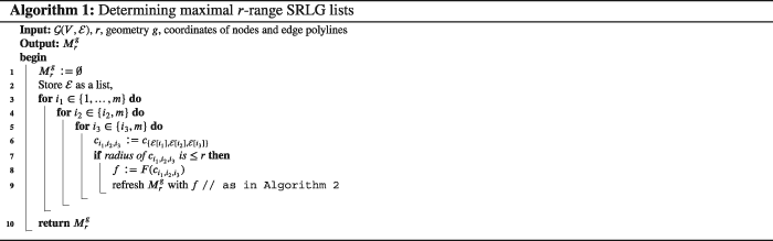
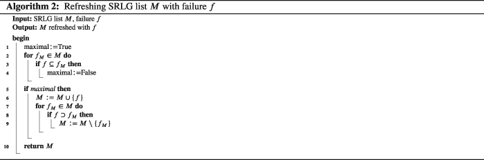
Secondly, according to Theorem , smallest enclosing disks can be computed in O(γ3) time both in the plane and on the sphere. Based on these, Algorithm 1 is presented, which is a straightforward basic polynomial algorithm. Here, the key idea is to maintain a list M′ of maximal failures detected so far while scanning through the link sets f covered by the smallest enclosing disks of at most 3 edges. If there is no fM ∈ M′ containing f, then f is appended to M′ and all fM ∈ M′ which are part of f are removed as presented in Algorithm 2. This process is called refreshing.
The following theorem gives a very loose bound on the complexity of calculating  .
.
Theorem 6.Algorithm 1 computes  in O(m3(γ3 + m4)) time.
  has O(m3) elements.
Proof.Based on Proposition , the algorithm is correct, it is computing  . There are O(m3) smallest enclosing disks to calculate, each in constant time. We claim that for each disk the calculation time of refreshing
  with the resulting failure (according to Algorithm 2) is O(m4 + γ3) in case of each disk, because after the computation of the smallest enclosing disk in O(γ3) time and determining f in O(m) time, we require to compare f with O(m3) link sets, and each comparison can be done in O(m)
time.
with the resulting failure (according to Algorithm 2) is O(m4 + γ3) in case of each disk, because after the computation of the smallest enclosing disk in O(γ3) time and determining f in O(m) time, we require to compare f with O(m3) link sets, and each comparison can be done in O(m)
time.
3.3 On improved complexity bounds
The results from the previous section can be easily improved using parametrization and some computational geometric tricks.
The first observation is that for any meaningful radius of the disk failure most of the network will remain intact. However, failures with the same radius taking place in a crowded area tend to take down more equipment than the ones in sparsely inhabited areas. This motivates the introduction of a graph density parameter:
Definition.For every  , let ρr be the maximum number of edges which can be destroyed by a disk with radius at most r.
This ρr is considered to be small in case of small r values. Another observation is that there are not many more network edges than nodes. This is formalized in the upcoming Claim .
Informally speaking, we denote the set of crossing points of the edges by X. A more formal definition follows.
Definition.Let X be the set of points P in the plane on which no node element of V lies and there exist at least 2 edges which have polylines having a finite number of common points crossing each other in P. Let x = | X|.
Despite the fact that on arbitrary graphs x can be even O(n4), in backbone network topologies typically x ≪ n because a node is usually installed if two cables are crossing each other. This gives us the intuition that G is “almost” planar, and thus it has few edges.
Claim 1.The number of edges in G is O(n + x). More precisely for n ≥ 3 we have m ≤ 3n + x − 6.
Proof.If  is embedded in the plane, do the following. Let G0(V ∪ X, E0) be the planar graph obtained from dividing the polylines of edges of G at the crossings. Since every crossing enlarges the number of edges at least by two, |E0 | ≥ m + 2x. On the other hand, |E0 | ≤ 3(n + x) − 6 since G0 is planar. Thus m ≤ | E0 | − 2x ≤ 3n + x − 6.
If  is embedded in the sphere, we can project it to the plane with stereographic projection, repeat the former arguments then apply an inverse projection to the sphere.
A third trick relies on the fact that in practice  is O(n) (as presented in planar case in 25), thus in Algorithm 2 typically there have to be done only O(n) comparisons. Thus, we introduce a third parameter:
Definition.Let λ be the maximum cardinality of the list of maximal failures detected so far in Algorithms 1, 3, and 4, respectively.
Combining the former three observations, a lower parametrized complexity can be achieved:
Theorem 7.Algorithm 1 computes  in O((n + x)3(n + x + λρr + γ3) time.
Proof.Based on Proposition , the algorithm is computing  . There are O((n + x)3) smallest enclosing disks to calculate, each in constant time. We claim that for each disk the calculation time of Algorithm 2 is O((n + x)3ρr + γ3) in case of each disk, because after the computation of the smallest enclosing disk in O(γ3) and determining f in O(n + x) we require O(λ) comparisons of link sets (i.e., pairs of possible maximal failures), and each comparison can be done in O(ρr)
time.
. There are O((n + x)3) smallest enclosing disks to calculate, each in constant time. We claim that for each disk the calculation time of Algorithm 2 is O((n + x)3ρr + γ3) in case of each disk, because after the computation of the smallest enclosing disk in O(γ3) and determining f in O(n + x) we require O(λ) comparisons of link sets (i.e., pairs of possible maximal failures), and each comparison can be done in O(ρr)
time.
Corollary will give more intuitive bounds on the running time of Algorithm 1.
Definition.Let diam be the geometric diameter of the network.
Proposition 8.Based on simulation results from Section VI of 25, in case of backbone networks, ρr is proportional to  in the interval (0, diam/2], where diam is the geometric diameter of the network.
Corollary 9.(corollary of Theorem ). If both x and λ are O(n), Algorithm 1 computes  in O(n3(nρr + γ3)) time. If, in addition, γ is O(1) and ρr is O(r/diam), Algorithm 1 computes
  in
in  time.
time.
Corollary proposes that  can be determined in quartic time of n in practice. On the other hand, Algorithm 1 has its limits of speed: because of the three nested for-loops, it runs in Ω(n3) time. In order to achieve better results, the algorithm would have to be changed. For the planar case, Reference 25 gives an algorithm which runs in
  time for γ = 1 (i.e., the edges are considered as line segments there). Furthermore, we are convinced that an algorithm with parametrized running time near-linear in network size could be achieved for determining
  (and also for determining
  and
and  , despite the fact that they can be computed based on very different theories). However, presenting this kind of algorithm would exceed the limits of this paper.
4 APPROXIMATE ALGORITHMS AND IMPLEMENTATION ISSUES
It is always good to have fast precise polynomial algorithms for solving a given problem. However, this approach also has some disadvantages: (1) the lower complexity a precise algorithm for determining a maximal circular SRLG list has, the harder to implement and prove its correctness and complexity; (2) designing algorithms for computing different types of maximal SRLG lists need totally different mathematics. Moreover, in most cases, the available geographical data of networks are inaccurate. Adding this fact to the inconveniences of the precise approach results into the idea of designing some approximate algorithms that are able to compute these lists with enough precision.
The main idea behind this class of algorithms that instead of keeping the original shape and size of the disaster area and taking in count all the infinitely many possible disaster centers, we slightly overestimate the disaster, letting us detect all the same (or occasionally a bit larger) hit link sets while going through only a finite number of centers.
4.1 Approximate algorithms for circular disk failures
In this section, we present an approximate approach suitable for computing all types of maximal SRLG lists defined in Section 2.
Definition.For a point P (in the plane or on the sphere) and node v ∈ V, let the node-distance couple be [v, d(v, P)], where d(v, P) is the distance between v and P. Let e(P) be the list consisting of the link-distance pairs of all links e ∈ ℰ, sorted according to the lexicographical order of the links. Let e(P)hit be the sorted list of links not further from P than r.
Proposition 10.For a given point P, both e(P) and e(P)hit can be computed in O((n + x)γ) time.
Clearly, both node-distance lists and edge-distance lists can be determined quickly. The plan is to determine these lists for enough points which are also placed well enough to be able to determine the maximal SRLG lists based on these node-distance and edge-distance lists.
Definition.Let  denote the set of points P for which we want to construct the link-distance lists e(P).
Let us stick to planar geometry for a moment. Intuitively, we can calculate  by including the grid points of a sufficiently fine grid (let us say containing 1 km × 1 km squares) in
  . On the sphere, we should choose a similar nice covering. It is possible that we have some extra short links, thus for calculating the k-node and k-link list we should include some extra points in
  . For example, by adding some random points of polylines of each edge and some point near every node, we can solve this issue.
Definition.Let  be the maximal distance of any geometric location from the (closed) convex hull of the geometric embedding of graph G to the closest point of set
  , that is,
  .
.
Definition.Taking two sets E1 and E2, we denote the relationship of the sets with E1 ⊒ E2 if and only if for all e2 ∈ E2 there exists an e1 ∈ E1, such that e1 ⊇ e2.
Algorithm 3 is an example approximate algorithm for determining  .
.
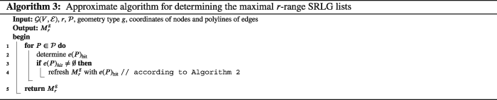
Theorem 11.The resulting list  of running Algorithm 3 is determined by the algorithm in
 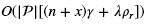 time. Furthermore,
  .
.
Proof.Regarding the complexity, for an element P of  we have to construct e(P)hit, which can be done in O((n + x)γ) time, then refresh the list of suspected maximal failures with e(P)hit in O(λρr), since the list contains at most λ ordered lists consisting of at most ρr edges.
On the other hand,  is immediate, since the algorithm investigates only a subset of disks with radius r, while for every point t in the r-neighborhood of conv(G), there exists a
  such that disk
  , yielding
  , from which the proof follows.
Using the fact that the shape of the disasters is a closed disk, we get the following corollary:
Corollary 12.
 , for any fixed network.
Corollary 13.(of Theorem ).  . Furthermore, if both x and λ are O(n), the resulting list
  of running Algorithm 3 is determined by the algorithm in
  time. If in addition, γ is O(1) and ρr is
  is determined by Algorithm 3 in
  time.
time.
Based on Theorem , if one wants to protect disasters caused by disks with radius r, it is only necessary to run Algorithm 3 initializing the radius as  .
.
Comparing Corollaries and , we can see that despite the fact that the approximate Algorithm 3 is much simpler to implement, and taking into account that disasters are not precisely circular and the chosen radius is arbitrary, it clearly outperforms the precise Algorithm 1.
4.2 Approximate algorithms for disasters with arbitrary shape
Understanding how to deal with circular disk failures is a good start; however, one should consider other disaster shapes too. In 28, it is proven that, in a similar problem setting (the model of 28 considers that a link is hit by a disaster exactly if at least one of its endpoints is inside the disaster region. We believe our failure model is more realistic), there are a polynomial number of maximal failures caused by disasters having elliptic or polygonal (e.g., rectangular or equilateral triangular) shape. Again, as engineering fast precise algorithms for determining SRLG lists similar to Mr, Mk or Ml but for arbitrary disaster shapes instead of a circle is not trivial, we are going to discover the possibilities of approximate algorithms similar to the one described for determining Mr. In short, while the disk is invariant to rotation, now one should consider also the different orientations of the fixed shape. We shall discretize the continuous rotation of the shapes via taking only a possible orientations of the shape:
Definition.Let Fr be a set of non-self-intersecting closed polytopes embedded in the plane having boundaries consisting of line segments and arcs, for which (1) every f1, f2 ∈ Fr, f1 can be moved into f2 via a translation and a rotation, and (2) the smallest fitting disk of any f ∈ Fr has a radius of r.
Let  consist of the elements f of Fr, each f extended (as
  ) with the smallest
  -neighborhood of f.
 be the consisting of the elements f′ of
  , each f′ extended as f ′ ′ with the smallest da, T-neighborhood of f′ (where distance da, T is a function of the extended shape f′, the number of orientations of the shape considered a, and the center of rotation T ∈ intf) in such a way that:
 (1)
(1)By the former definition, we have the following. For any possible place and orientation of a disaster with shape f, in which f intersects at least a network element, there exists a  and an orientation of the extended disaster shape f ′ ′ for which the area destroyed by f ′ ′ contains the area destroyed by f. This also holds if the orientation is taken from among the a investigated orientations. Thus the edge set hit by f ′ ′ is a superset of the edge set hit by f.
Proposition 14.
 .
.
Definition.Let ϕ denote the number of line segments and arcs needed to describe a shape from Fr. Let ϱr be the maximal number of edges an f ∈ Fr can hit.
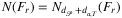
Definition.For geometry type g ∈ {p, s}, let denote the set of maximal failures caused by disasters from Fr and N(Fr) by  and
and  , respectively.
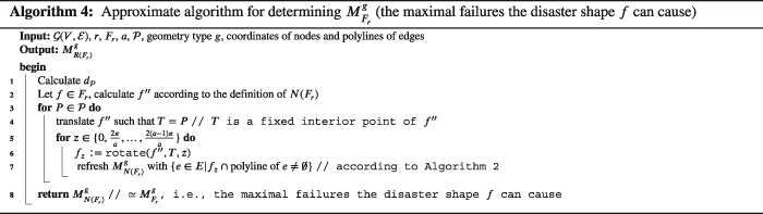
Algorithm 4 is an example approximate algorithm for determining  .
.
Theorem 15.The resulting list  of running Algorithm 4 is determined by the algorithm in
 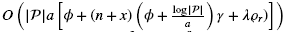 time if the original failure shape f is convex. Furthermore, for any given network,
  .
.
Proof.Clearly, the algorithm computes  . Based on Proposition proposing that as
  and a → ∞, the necessary inflation of the original shape f tends to 0, we also can see that for any given network,
 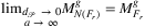 .
.
Regarding its complexity, we can argue as follows.
To calculate  , we observe that all the points in Nr(G) (the smallest r-neighborhood of the convex hull of G) maximizing the distance from
  lie on the intersection of at least 3 Voronoi cells computed on point set
  , restricted to Nr(G), and the outer region of Nr(G) taken as an extra cell. The Voronoi regions of
  can be computed in
  time both in the plane and on the sphere (plane: Section 7.2 in 5, sphere: special case of Corollary 2 in 18). Using Claim , one can see that the number of line segments and arcs (or geodesics on the sphere) needed to describe Nr(G) is O((n + x)γ), thus we claim the total complexity of computation and description the modified Voronoi diagram described before is
  . Based on the graph representation of the diagram one can determine
  in the proposed complexity.
We claim that Line 2 can be done in O(ϕ) time if f is convex. In case of non-convex failure shapes, f calculations can become more complicated (e.g., holes in f can disappear in f ′ ′), but clearly, f ′ ′ can be determined in time polynomial in ϕ in this case too.
For a given  , translation of f (Line 4) can be done in O(ϕ)
time.
, translation of f (Line 4) can be done in O(ϕ)
time.
For a given  and
and  , rotation (Line 6) can be done in O(ϕ)
time.
, rotation (Line 6) can be done in O(ϕ)
time.
For a given point and direction, Line 7 needs O((n + x)ϕγ + λϱr) operations, as follows. For every edge e ∈ ℰ one has to check whether its polyline el intersects the boundary of fz or if not, is el situated entirely in fz, both can be checked in O(ϕγ). Then, refreshing  with the edge set hit by fz can be done in O(λϱr) time, since edges are stored in ordered lists.
We can conclude that Algorithm 4 is correct and runs in the proposed complexity.
Algorithm 4 clearly runs in time polynomial in the input size (even for non-convex disaster shapes f), and can be applied for a wide variety of disaster shapes.
Corollary will offer a more intuitive complexity result on Algorithm 4:
Proposition 16.Since any f ∈ Fr can be covered with a disk having a radius r, ϱr ≤ ρr. Based on Proposition , this also means that ϱr is  in case of backbone networks.
Corollary 17.If the number of edge crossings x is O(n), parameters γ and ϕ are O(1), and  is chosen to be O(a), the resulting list
  of running Algorithm 4 is determined in
  time. If, in addition, λ is O(n), and ϱr is
  , the runtime is
  .
.
If we compare Corollaries and , we can see that unless the shape f of disasters is very complicated, the only real additional complexity compared to the circular disk failure case arises from the fact that that usually f is not invariant to rotation.
Comparing Corollaries and , we can see that although the approximate Algorithm 3 handles the much more complex problem induced by disasters having an arbitrary given shape f, it has a lower complexity compared to the precise Algorithm 1 dealing with only circular disasters, showing the strength of the proposed framework of approximate algorithms.
5 SIMULATION RESULTS
In this section, we present numerical results that validate our approximate approach for circular disk failures presented in Section 4.1, and demonstrate the use of the proposed algorithms on some realistic physical networks. The algorithm was implemented in Python 3.5 using various libraries. Distance functions were implemented from scratch. No special efforts were made to make the algorithm space or time optimal. Run-times were measured on a commodity laptop with Core i5 CPU at 2.3 GHz with 8 GB of RAM. The output of the algorithm is a list of SRLGs such that no SRLG contains the other.
We interpret the input topologies in two ways: polygon, where links are polygonal chains, and line, where the corner points of the polygonal links are substituted with nodes (of degree 2). Here links are line segments.
5.1 Extreme geographical extension makes difference
We found that running times for spherical representations were ∼2 times slower than the planar ones in case of most networks (see Table 2). The only exception is when the network has an extreme geographic extension (e.g., AboveNet), in this case, the obtained SRLG lists tend to be longer (Figure 3 demonstrates this in case of k-link lists) causing a slight increase both in the parameter λ and in the running time.
 )
)| |V| | |ℰ| | Planar runtime | Spherical runtime | |||||
|---|---|---|---|---|---|---|---|---|
| Name | Polygon | Line | Polygon | Line | Polygon | Line | Polygon | Line |
| AboveNet | 9 | 22 | 15 | 28 | 232 | 156 | 410 | 757 |
| LambdaNet | 10 | 33 | 10 | 33 | 282 | 225 | 444 | 410 |
| GARR (Italy) | 16 | 16 | 18 | 18 | 107 | 92 | 204 | 187 |
| GTS (Hungary) | 14 | 15 | 39 | 26 | 175 | 146 | 311 | 291 |

 compared to
  for small l values. B,
  compared to
  for all possible l values. C, Best Mercator projection of AboveNet
Another issue which can be noticed is related to the achievable preciseness using the approximate approach. Based on Theorem , running time is proportional to  ; given this and the running times collected in Table 2, we can deduce that if the drop of price of computation power remains for an additional short time period, one will be able to run these simulations even at home for huge
  (e.g.,
  , which number is approximately the Earth's surface in
  ), yielding a high precision. Note that Algorithm 3 could be easily parallelized.
The k-link list is chosen as an illustrative example in Figure 3. In Figure 3A,B, we can see that for k = 1, there are listed all the single link failures. For k ≥ 2, there is a higher chance on the sphere for k links to be “close” to each other than on the plane, thus  . This phenomenon might appear because mapping the sphere to the plane intuitively lets fewer edges to be next or close to each other. As the number of links in the SRLGs l increases,
  first increases too, then after plateauing it starts to decrease, which is just a rephrasing of the intuition that there are the most possible scenarios of a disk hitting exactly l links when l ≃ m. Finally,
  , because there is only one possibility of hitting all the links.
The obtained SRLG lists are different for the two geometries, thus it makes sense to use the much more precise spherical model.
5.2 Cardinality of SRLG lists induced by disasters with a shape of circular disk
In this section, a brief overview is given on the typical cardinality of the proposed (planar) l-link, k-node and r-range lists. The chosen example topology is the 28_optic_eu drawn in Figure 4C, and having 19 and 28 vertices, and 32 and 41 edges, in polygon and line case, respectively. On Figure 4B, one can see that all  and
and  are reasonably small, for smaller values of the measure.

 compared to
  for for all possible l values. B,
  compared to
  and
and  for small l/k/r values. C, A planarization of 28_optic_eu
 equals the number of edges by definition, and for l ∈ {1, …, 5}, 1.2 * l times the number of edges is a good approximation for the cardinality of the list. This linear increase then flattens out,
  reaching its maximum at l = 10 and 15 in chain and line case, respectively, then slowly decreases to 1, while l reaches the number of edges.
The overall dynamics of graphs of  are the same as that of
  ; however, the increase in the number of SRLGs is more moderate for small k values: (k + 1.2) times the number of nodes is a good approximation for
  in the area of small k values, and the cardinality culminates at
  and
and  in the chain and segment cases, respectively.
It is easy to see that  equals the number of nodes and edge crossings, the worst places of disasters having small geographical extensions being at nodes and edge crossings. In case of this topology and the chosen radii, the maximum cardinality of
  was reached at 180 and
  for the chain and segment cases, respectively, with values of 48 and 133.
5.3 When can we neglect the curvature of the Earth?
An important question is that, in practice, under which geographic extension of the network can one say that, in the viewpoint of SRLG enumeration, it is practically indifferent whether we consider a spherical or a planar representation of the network. In other words, focusing now only on lists Mr, the question is that under which size of the physical network will  and
and  (maximal link sets which can be hit by a single circular disk with radius r, in the plane and on the sphere, respectively) be the precisely the same. The answer depends not only on the physical size, but also on the characteristics of the network itself: it can represent a dense metropolitan backbone network with multiple nodes close to each other, but it can also be geographically very sparse. Keeping in mind that in metropolitan areas there can be many more differences, we took network AboveNet (Figure 3C), and its shrunk instances, where AboveNet/c means that we rotated AboveNet such that the average lat and lon coordinates are both 0, then we divided each coordinate by c. We were interested in the smallest possible shrinking ratio, for which
  .
.
We used  (the ratio of SRLGs, which are present in only one of
  and
and  ) as a similarity measure: if ℳ(r) is close to 1, it means the two lists are very different, while if it is close to 0, it means there are few differences. We set r = 8 to be a bit larger than half of the diameter of the current network, r = 0 to be a small radius, the rest of the r values were linearly interpolated.
Figure 5 shows that, while in case of AboveNet,  and
and  are almost entirely different for many values of r, the tendency is that ℳ(r) decreases as the physical size of the network decreases, which nicely fits the intuition. Surprisingly, ℳ(r) is not 0 for every range r even for AboveNet/300, which corresponds to the case when the approximate network diameter is
  , AboveNet/400 (having a diameter of approx.
  ) being the most spread out instance where
  and
and  are the same for all investigated r ranges.

 and
and  , that is,
As a rule of thumb, we can deduce that the difference between the planar and spherical representations of the network can result in different SRLG lists even in the case of networks having a geographic extension as small as  .
.
6 CONCLUSION
We investigated the problem of generating SRLG lists of networks. We found that the known precise low-polynomial SRLG generating techniques can be modified in order to fit the spherical geometry, allowing us to generate SRLG lists with more precision. A framework of easy-to-implement approximating algorithms for determining the SRLG lists in both planar and spherical representation was also presented.
In our experience, SRLG lists generated using the spherical representation of the networks are different from the planar ones, and also they tend to be longer, especially in case of extreme geographical extension. In the case of our implementation, enumerating SRLG lists in case of spherical representations was typically 2 times slower than in the planar case. The difference between the planar and spherical representations of the network can result in different SRLG lists even in the case of networks having a geographic extension as small as  .
.
While in most of our study, we supposed the disasters destroy the network in an area of a circular disk, some results were generalized to essentially arbitrary disaster shapes.
APPENDIX A: DETERMINING SMALLEST ENCLOSING DISK OF LINE SEGMENTS OR GEODESICS IN O(1) TIME
Proof of Lemma 3.For planar geometry, this problem is already solved, see Theorem 3 of paper 25. It remains to prove it in case of spherical embedding.
Let e1, e2, e3 be three geodesics on the sphere. The endpoints (pi1, pi2) are given by Cartesian coordinates (xi1, yi1, zi1), (xi2, yi2, zi2). Let pi3 be an arbitrary point inside ei. Points pi1, pi2 and pi3 determine the great circle on the sphere containing geodesic ei.
We will project geometric objects on the sphere to the plane using the stereographic projection from the north pole, which has the property that the image of a spherical circle will be a circle on the plane, or in special case, if it contains the north pole, its image is a line 22. Note that for the sake of simplicity it is assumed that no great circle investigated crosses the north pole.
Projecting the 9 spherical points onto the plane, we receive qij points given by Cartesian coordinates  . We denote the images of e1, e2, e3 by arcs f1, f2, f3. Calculating the radius and center point of the containing circle ci for arc fi requires constant number of coordinate geometric steps. Let (x1, y1), (x2, y2), (x3, y3) and r1, r2, r3 be the Cartesian coordinates of the center of containing circles, and radii, respectively.
The smallest enclosing disk cH on the sphere has an image c′H on the plane. However, the parameters of c′H are different from the parameters of cH, and the images of the fitting points of cH and ei are the fitting points of c′H and fi. That inspires the plan to find all the fitting circles of fi (i.e., those which have exactly one common point with each fi or which have one common point with two of them and containing the third) on the plane, project them back onto sphere and select the smallest among them, as that is the smallest enclosing disk of e1, e2, e3. Thus, we need to find the potential best fitting circles in the plane.
It is possible that the disk fits for two arcs and includes some points of the third. We can choose two arbitrary arcs in 3 ways. Choosing f1, f2 we must calculate the distance of the two arcs and use it as the diameter of the potential disk. On each arc, the distance is determined by an inside point or one of the boundary points. Calculating the distance of two points, a point and a circle or two circles have both constant complexity. So, in this case, 3 · 32 · O(1) calculations are required.
If the smallest disk touches all of the arcs there are also more different cases. Each arc can be touched on a boundary point or on an inside point (33 cases). Fortunately, fitting a circle is already solved in all of the cases and these are known as the problems of Apollonius 4.
If the smallest enclosing disk touches all three arcs f1, f2, and f3, we have three cases for each arc fi: the disk either touches the arc in an interior point or at one of its endpoints. In the former case let (x1, y1) and ri be the Cartesian coordinates of the center point and radius of the containing circle of arc fi, respectively. In the latter case, let (x1, y1) be coordinates of the endpoint itself, while let ri be 0. Numbers s1, s2, and s3 are ±1 representing that the fitting circle touches on the outside or on the inside of the containing circles of c1, c2, and c3 (23 different possibilities to be checked in each case). Parameters xs, ys, and rs of the fitting C circle can be calculated by solving the following system of equations 2:

The system is quadratic, thus it can be solved in a constant number of arithmetic calculations. The complexity of these calculations all together are 33 · 23 · O(1).
After finding the 33 · 23 + 3 · 32 possible smallest disks, we must project them back to the surface of the sphere. We are allowed to use only the two endpoints of an arbitrary diameter from each possible circle. This requires 2 · 35 coordinate transformations  .
.
Finding the minimal radius of potential disks requires 35 − 1 comparisons between diameters. Using this method the minimal disk for e1, e2, e3 can be determined in O(1) time. However, the algorithm could be improved by using pre-computations for the edges, excluding some possible disks already on the plane instead of transforming back or fixing si in case of boundary points. Note that only a constant number of basic arithmetic functions ( ) were used during the computation.