Volume 90, Issue 4 pp. 1518-1536

RESEARCH ARTICLE

Open Access

Bloch simulator–driven deep recurrent neural network for magnetization transfer contrast MR fingerprinting and CEST imaging

Munendra Singh,

Munendra Singh

Division of MR Research, Department of Radiology, Johns Hopkins University, Baltimore, Maryland, USA

Search for more papers by this author

Shanshan Jiang,

Shanshan Jiang

Division of MR Research, Department of Radiology, Johns Hopkins University, Baltimore, Maryland, USA

Search for more papers by this author

Yuguo Li,

Yuguo Li

Division of MR Research, Department of Radiology, Johns Hopkins University, Baltimore, Maryland, USA

Search for more papers by this author

Peter van Zijl,

Peter van Zijl

Division of MR Research, Department of Radiology, Johns Hopkins University, Baltimore, Maryland, USA

F.M. Kirby Research Center for Functional Brain Imaging, Kennedy Krieger Institute, Baltimore, Maryland, USA

Search for more papers by this author

Jinyuan Zhou,

Jinyuan Zhou

orcid.org/0000-0002-6684-7920

Division of MR Research, Department of Radiology, Johns Hopkins University, Baltimore, Maryland, USA

Search for more papers by this author

Hye-Young Heo,

Corresponding Author

Hye-Young Heo

[email protected]

orcid.org/0000-0002-7297-2015

Division of MR Research, Department of Radiology, Johns Hopkins University, Baltimore, Maryland, USA

F.M. Kirby Research Center for Functional Brain Imaging, Kennedy Krieger Institute, Baltimore, Maryland, USA

Correspondence

Hye-Young Heo, Division of MR Research, Department of Radiology, Johns Hopkins University School of Medicine, Baltimore, MD 21287, USA.

Email: [email protected]

Search for more papers by this author

Munendra Singh,

Munendra Singh

Division of MR Research, Department of Radiology, Johns Hopkins University, Baltimore, Maryland, USA

Search for more papers by this author

Shanshan Jiang,

Shanshan Jiang

Division of MR Research, Department of Radiology, Johns Hopkins University, Baltimore, Maryland, USA

Search for more papers by this author

Yuguo Li,

Yuguo Li

Division of MR Research, Department of Radiology, Johns Hopkins University, Baltimore, Maryland, USA

Search for more papers by this author

Peter van Zijl,

Peter van Zijl

Division of MR Research, Department of Radiology, Johns Hopkins University, Baltimore, Maryland, USA

F.M. Kirby Research Center for Functional Brain Imaging, Kennedy Krieger Institute, Baltimore, Maryland, USA

Search for more papers by this author

Jinyuan Zhou,

Jinyuan Zhou

orcid.org/0000-0002-6684-7920

Division of MR Research, Department of Radiology, Johns Hopkins University, Baltimore, Maryland, USA

Search for more papers by this author

Hye-Young Heo,

Corresponding Author

Hye-Young Heo

[email protected]

orcid.org/0000-0002-7297-2015

Division of MR Research, Department of Radiology, Johns Hopkins University, Baltimore, Maryland, USA

F.M. Kirby Research Center for Functional Brain Imaging, Kennedy Krieger Institute, Baltimore, Maryland, USA

Correspondence

Hye-Young Heo, Division of MR Research, Department of Radiology, Johns Hopkins University School of Medicine, Baltimore, MD 21287, USA.

Email: [email protected]

Search for more papers by this author

First published: 15 June 2023

https://doi.org/10.1002/mrm.29748

Citations: 9

Share a link

Email
Wechat
Bluesky

Abstract

Purpose

To develop a unified deep-learning framework by combining an ultrafast Bloch simulator and a semisolid macromolecular magnetization transfer contrast (MTC) MR fingerprinting (MRF) reconstruction for estimation of MTC effects.

Methods

The Bloch simulator and MRF reconstruction architectures were designed with recurrent neural networks and convolutional neural networks, evaluated with numerical phantoms with known ground truths and cross-linked bovine serum albumin phantoms, and demonstrated in the brain of healthy volunteers at 3 T. In addition, the inherent magnetization-transfer ratio asymmetry effect was evaluated in MTC-MRF, CEST, and relayed nuclear Overhauser enhancement imaging. A test–retest study was performed to evaluate the repeatability of MTC parameters, CEST, and relayed nuclear Overhauser enhancement signals estimated by the unified deep-learning framework.

Results

Compared with a conventional Bloch simulation, the deep Bloch simulator for generation of the MTC-MRF dictionary or a training data set reduced the computation time by 181-fold, without compromising MRF profile accuracy. The recurrent neural network–based MRF reconstruction outperformed existing methods in terms of reconstruction accuracy and noise robustness. Using the proposed MTC-MRF framework for tissue-parameter quantification, the test–retest study showed a high degree of repeatability in which the coefficients of variance were less than 7% for all tissue parameters.

Conclusion

Bloch simulator–driven, deep-learning MTC-MRF can provide robust and repeatable multiple-tissue parameter quantification in a clinically feasible scan time on a 3T scanner.

1 INTRODUCTION

Saturation-transfer MRI provides unique and flexible contrast mechanisms, including semisolid magnetization transfer contrast (MTC) and CEST, which enable indirect detection of MR-invisible protons bound to macromolecules (e.g., semisolid proteins and lipid bilayers of myelin) or water-exchangeable solute protons (e.g., mobile proteins and peptides), respectively.^1-4 MTC imaging is highly sensitive to demyelination, inflammation, and edema and has shown promise for evaluating white-matter diseases, such as multiple sclerosis and traumatic brain injury.^5-7 However, MTC measured by a conventional MT ratio (MTR) metric depends on multiple parameters, including semisolid proton concentration, average exchange rate of bound water and exchangeable protons, and free water relaxation properties.^8-10 In addition, the ratio is affected by imaging scan parameters, such as RF irradiation frequency, saturation field strength, and duration. To improve the specificity and reproducibility of MTC, quantitative magnetization-transfer (MT) imaging analysis procedures have been used to estimate intrinsic tissue properties that are independent of the choice of acquisition parameters, most commonly by fitting acquired MTC-weighted images to a biophysical two-pool exchange model.^{3, 11-13} However, the fitting-based approach is often computationally intensive, susceptible to being stuck at local minima, and dependent on the number of fitting parameters, initial fitting values, and boundary conditions, often leading to poor quantification accuracy and computational efficiency.

Although MTC has a broad absorption lineshape of the semisolid macromolecule-bound protons over a wide range of frequencies, CEST contrast is based on RF irradiation applied at a frequency offset specific for certain exchangeable protons. Amide proton transfer (APT) is one type of CEST contrast for a large group of amide protons (-NH) with an average chemical shift of about 3.5 ppm downfield from water. APT-weighted MRI has shown great potential in the diagnosis of many pathologies, such as cancer, stroke, and neurodegenerative disease.^14-29 When applying RF saturation at 3.5 ppm for APT imaging, however, free bulk water and semisolid macromolecular protons may also be saturated due to overlap in the chemical shift, leading to an inevitable interference with the desirable APT contrast. Although a conventional MTR asymmetry (MTR_asym) analysis can largely remove symmetric, direct water saturation and MTC effects, the APT-weighted (APTw) signal, measured by the MTR asymmetry analysis, is still confounded by inherent MT asymmetry, both from the relayed nuclear Overhauser effect (rNOE) in mobile macromolecules upfield from water and asymmetry in the semisolid MTC.^30-33 To make matters worse, the MTR asymmetry and/or rNOE effects are weighted by the choice of RF saturation parameters, thus reducing the specificity of APTw contrast.^{16, 34-36}

Recently, fast and quantitative MTC and CEST imaging techniques have been proposed by integrating an RF saturation scheme with MR fingerprinting (MRF).^37-41 Various RF saturation parameters are applied, which create distinct signal evolutions for different tissue properties. For MRF reconstruction, a pattern-matching algorithm is typically needed to determine different tissue-type parameters against a precalculated dictionary created by Bloch simulations with a large range of tissue parameters.³⁸ However, depending on the sequence type, the number of tissue properties, and the granularity of the tissue property values, the dimension or size of the dictionary is exponentially increased, which inevitably leads to an intensive computation time for dictionary generation and MRF reconstruction. To reduce the computational burden for MRF reconstruction, deep learning–based reconstruction techniques have been developed by learning the mapping relationship between MRF signals and tissue properties.^{37, 39-43} To improve reconstruction accuracy and generalization performance, the training data set must be highly sampled with a wide range of tissue-parameter combinations, which is extremely computationally expensive. In addition, optimization of the MRF acquisition schedule is very important to accelerate data acquisition and improve accuracy of the tissue-parameter estimation.^{43, 44} However, repeatedly generating a dictionary or training data set for each MRF schedule tested incurs a very high and impractical computational cost. In this study, a unified deep-learning architecture that included an ultrafast Bloch simulator and tissue-parameter reconstruction was developed to address these issues. A deep Bloch simulator was designed to generate a large training data set in a short time. A hybrid deep-learning model combined with a recurrent neural network (RNN) and a convolutional neural network (CNN) was proposed to improve the accuracy of MTC-MRF reconstruction (water proton and semisolid macromolecular proton parameters, such as relaxation time, pool size ratio, and exchange rate). The performance of the hybrid neural network was evaluated on numerical phantoms with known ground truths and cross-linked bovine serum albumin phantoms. The proposed framework was demonstrated on healthy volunteers and compared with previous reconstruction methods,^{40, 45} including a fully connected neural network (FCNN) and Bloch fitting approaches. In addition, a test–retest study was performed to evaluate the repeatability of the tissue parameters estimated from the deep-learning framework.

2 THEORY

The Bloch simulator and MTC-MRF reconstruction are based on a two-pool exchange model. The dependence of tissue and scan parameters is captured by forward and inverse models derived from two-pool Bloch equations.^{3, 40, 46}

2.1 Steady-state two-pool MTC model

The MTC process can be described by a two-pool exchange model: free bulk water proton (w) and semisolid macromolecular proton (m) pools. Two-pool signal profiles were generated with a pseudorandomized RF saturation and acquisition parameters consisting of RF saturation strength (B₁), saturation time (Ts), frequency offset (Ω), TR or relaxation delay time (Td), as shown in Figure 1A,B. A steady-state MTC signal (

{S}_{\mathrm{MTC}}^{\mathrm{ss}}

) assuming a long Ts and TR is derived as follows³:

{S}_{\mathrm{MTC}}^{\mathrm{ss}}\left({\omega}_{\mathrm{off}},{\omega}_1\right)=\frac{\alpha_1}{\alpha_2}

(1)

{\alpha}_1=\frac{1}{T_1^{\mathrm{m}}}\left({k}_{\mathrm{m}\mathrm{w}}{M}_0^{\mathrm{m}}{T}_1^{\mathrm{w}}\right)+{R}_{\mathrm{rf}}+{k}_{\mathrm{m}\mathrm{w}}+\frac{1}{T_1^{\mathrm{m}}}

(2)

\begin{array}{cc}{\alpha}_2& =\left({k}_{\mathrm{m}\mathrm{w}}{M}_0^{\mathrm{m}}{T}_1^{\mathrm{w}}\right)\left({R}_{\mathrm{rf}}+\frac{1}{T_1^{\mathrm{m}}}\right)\\ {}& \kern1em +\left[1+{\left(\frac{\omega_1}{\omega_{\mathrm{off}}}\right)}^2\right]\left(\frac{T_1^{\mathrm{w}}}{T_2^{\mathrm{w}}}\right)\left({R}_{\mathrm{rf}}+\frac{1}{T_1^{\mathrm{m}}}+{k}_{\mathrm{m}\mathrm{w}}\right)\end{array}

(3)

where

{T}_1^{\mathrm{m}}

and

{T}_2^{\mathrm{m}}

are, respectively, longitudinal relaxation time and transverse relaxation time of a semisolid macromolecular proton pool; k_mw is the proton exchange rate from pool m to pool w;

{M}_0^{\mathrm{m}}

is the equilibrium magnetization of a pool m; ω_off is the frequency offset of the RF saturation, defined as ω_{off =} γB₀Ω with

\Omega

in ppm; and ω₁ is the RF saturation amplitude, defined as ω₁ = γB₁. The value of

{M}_0^{\mathrm{w}}

is the equilibrium magnetization of a pool w;

{T}_1^{\mathrm{w}}

is longitudinal relaxation time; and

{T}_2^{\mathrm{w}}

is transverse relaxation time of free bulk water. Note that the ratio of semisolid macromolecular pool size to free water pool size (pool size ratio) is defined as F = 100% × (

{M}_0^{\mathrm{m}}

{M}_0^{\mathrm{w}}

), where

{M}_0^{\mathrm{m}}

is set to 1. The RF absorption rate (R_rf), which is the rate of loss of the longitudinal magnetization of the semisolid macromolecule pool, is dependent on the super-Lorentzian lineshape (g_m) as follows:

{R}_{\mathrm{rf}}={\omega}_1^2\uppi {g}_{\mathrm{m}}\left(\Delta \omega \right)

(4)

\Delta \omega ={\omega}_{\mathrm{off}}-{\Delta}_{\mathrm{mw}}

(5)

{g}_{\mathrm{m}}\left(\Delta \omega \right)=\sqrt{\frac{2}{\uppi}}\int_0^1\left(\frac{T_2^{\mathrm{m}}}{\mid 3{x}^2-1\mid}\right).{e}^{-2{\left(\frac{\Delta \omega {T}_2^{\mathrm{m}}}{\mid 3{x}^2-1\mid}\right)}^2}\mathrm{d}x

(6)

where Δ_mw is the radial frequency difference between the semisolid macromolecule and the free bulk-water proton pools. Note that a positive Δ_mw corresponds to the MTC lineshape center shifted upfield from the water resonance, whereas a negative Δ_mw corresponds to the MTC lineshape shifted downfield. The on-resonance singularity problem of the super-Lorentzian lineshape was avoided by extrapolating

{g}_{\mathrm{m}}\left(\Delta \omega \right)

signal.^{13, 47} The super-Lorentzian values were extrapolated from 1 kHz to the asymptotic limit and approximated by cubic spline method.

Details are in the caption following the image — **FIGURE 1**
Open in figure viewer PowerPoint

(A) Illustration of RF saturation–encoded magnetization-transfer contrast (MTC)–MR fingerprinting (MRF) sequence. A two-channel parallel transmission (pTX) was used to achieve continuous RF saturation at a 100% duty cycle. A variable density undersampling pattern with the elliptic-centric k-space ordering was used in a turbo spin-echo (TSE) sequence and a spectral presaturation with inversion recovery was used for fat-suppressed data acquisitions. (B) Example of B₁, Ts, Ω, and Td schedule for an MRF image acquisition. (C) MTC-MRF framework consisting of a deep Bloch simulator (deepBS-RNN) and a reconstruction network (Recon-RNN). The value of P_t represents ground-truth (GT) tissue parameters, and P'_t represents estimated tissue parameters from the Recon-RNN. The estimated tissue parameters (P'_t) and acquired ${T}_2^{\mathrm{w}}$ are fed to the pretrained deep Bloch simulator (deepBS) module as input to calculate baseline reference signals (Z_ref[±3.5 ppm] = 100%–MTC [±3.5 ppm]). ^‡Indicates pretrained neural networks. pTX, parallel transmission; SPIR, spectral presaturation with inversion recovery

2.2 Non-steady-state two-pool MTC model

For a non-steady-state (transient-state) signal evolution with short Ts and Td, the MTC signal (

{S}_{\mathrm{MTC}}^{\mathrm{ns}}

) can be described by^{34, 46, 48}

{S}_{\mathrm{MTC}}^{\mathrm{ns}}\left({\omega}_{\mathrm{off}},{\omega}_1,\mathrm{Ts}\right)=\left({M}_0^{\mathrm{w}}-{S}_{\mathrm{MTC}}^{\mathrm{ss}}\right){e}^{\uplambda \mathrm{Ts}}+{S}_{\mathrm{MTC}}^{\mathrm{ss}}

(7)

where

\begin{array}{cc}\lambda & =\frac{1}{2}\sqrt{{\left(\frac{1}{T_1^{\mathrm{m}}}+{R}_{\mathrm{rf}}^{\mathrm{m}}+{k}_{\mathrm{m}\mathrm{w}}-\frac{1}{T_1^{\mathrm{w}}}-{R}_{\mathrm{rf}}^{\mathrm{w}}-{k}_{\mathrm{w}\mathrm{m}}\right)}^2+4{M_0}^{\mathrm{m}}{k}_{\mathrm{m}\mathrm{w}}^2}\\ {}& -\frac{1}{2}\left(\frac{1}{T_1^{\mathrm{w}}}+{R}_{\mathrm{rf}}^{\mathrm{w}}+{k}_{\mathrm{w}\mathrm{m}}+\frac{1}{T_1^{\mathrm{m}}}+{R}_{\mathrm{rf}}^{\mathrm{m}}+{k}_{\mathrm{m}\mathrm{w}}\right)\end{array}

(8)

{R}_{\mathrm{rf}}^{\mathrm{w}}=\frac{\omega_1^2{T}_2^{\mathrm{w}}}{1+{\left({T}_2^{\mathrm{w}}{\omega}_{\mathrm{off}}\right)}^2},{R}_{\mathrm{rf}}^{\mathrm{m}}=\frac{\omega_1^2{T}_2^{\mathrm{m}}}{1+{\left({T}_2^{\mathrm{m}}{\omega}_{\mathrm{off}}\right)}^2}

(9)

where

{R}_{\mathrm{rf}}^{\mathrm{m}}

and

{R}_{\mathrm{rf}}^{\mathrm{w}}

are the rate of loss of the longitudinal magnetization by semisolid macromolecules and water pools, respectively. For a series of transient MTC-MRF acquisitions, varied RF saturation and acquisition parameters are dynamically applied. The transient MTC-MRF signal evolution can be described as follows:

{S}_{\mathrm{MTC}}\left(\Omega, {\mathrm{B}}_1,\mathrm{Ts},\mathrm{Td}\right)=\left[{M}_0^{\mathrm{w}}\left(1-{e}^{-\frac{\mathrm{Td}}{T_1^{\mathrm{w}}}}\right)-{S}_{\mathrm{MTC}}^{\mathrm{ss}}\right]{e}^{\lambda \mathrm{Ts}}+{S}_{\mathrm{MTC}}^{\mathrm{ss}}

(10)

The relaxation delay time in the absence of RF irradiation allows the longitudinal magnetization recovery, determining an initial state of the magnetization for the next dynamic scan. To solve an inverse problem of the two-pool Bloch equation, a neural network architecture was designed to learn the nonlinear relation between tissue properties and the MRF signal profiles derived from the analytical solution (Eq. [10]) of the transient MTC-MRF model.

3 METHODS

3.1 Bloch simulator network

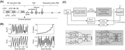
A bidirectional long-short-term memory (bi-LSTM)–based RNN was combined with convolutional and dense layers for the Bloch simulator (deepBS-RNN). The network had 64 hidden memory units of bi-LSTM as an input layer, one 1D convolutional layer with 128 channels, and two fully connected dense layers with 256 neurons in the middle, and one fully connected dense layer with 40 neurons as an output layer. For comparison of the performance of the deep-Bloch simulator, another Bloch simulator was designed using fully connected neural networks (deepBS-FCNN), which consisted of one fully connected input layer with five neurons, one fully connected output layer with 40 neurons, and four fully connected layers with 128 neurons in the middle. During the training of the Bloch simulators, the errors of the network outputs were calculated using the L1-norm loss function between ground truths and estimated MRF signal profiles, and then propagated back to the networks. The deep Bloch simulators were validated using a conventional two-pool Bloch simulation (BS) with ground truths. The Bloch simulations were performed in MATLAB (MathWorks, Natick, MA, USA) installed on a 64-bit Linux system (32-core, 3.75-GHz AMD processor, and 512 GB of memory).

3.2 Reconstruction network

A reconstruction network using RNN (Recon-RNN) was designed with bi-LSTM as an input layer, four 1D convolutional layers and four fully connected layers to extract the feature from MTC-MRF signals as middle layers, and one fully connected layer at an output layer. The bi-LSTM layer had 128 hidden memory units; each convolutional layer had 256 channels; each fully connected layer in middle had 512 neurons; and the last fully connected layer had four neurons. Rectified linear unit activation function was used to add nonlinearity after the bi-LSTM layer and each convolutional layer. A sigmoid activation function was used as the last activation function in the fully connected layer, and then the output values (tissue parameters) were de-normalized in their maximum to minimum range: k_mw: [100, 5] Hz; F: [2, 17] %;

{T}_2^{\mathrm{m}}

: [100, 1] μs; and

{T}_1^{\mathrm{w}}

: [3, 0.2] s. To evaluate the MTC asymmetry effect, an additional tissue parameter (Δ_mw: [4, 0] ppm) was estimated; hence, the fully connected layer had five neurons at the output. Note that

{T}_1^{\mathrm{m}}

was assumed to be 1 s due to a negligible contribution to the MTC signal.⁴⁹ Mean squared errors between ground-truth values and estimated tissue parameters (N = 4 or 5) were calculated as the loss function (Loss₁), as follows:

{\mathrm{Loss}}_1=\sum \limits_{i=1}^N\frac{{\left({P}_{\mathrm{t}}-P{\prime}_{\mathrm{t}}\right)}^2}{N}

(11)

where P_t is the ground truth and P'_t is the tissue estimate. After de-normalization, the estimated tissue parameters and the T₂ relaxation time of free bulk water (

{T}_2^{\mathrm{w}}

) were fed to a two-pool Bloch equation module to calculate MTC signal intensities at ±3.5 ppm with a B₁ of 1 and 1.5 μT. The second loss function (Loss₂) was calculated by averaging the sum of the squared difference between the ground-truth values and the estimated MTC signal intensities at 1 and 1.5 μT, respectively. The overall loss function was defined as

L={\mathrm{Loss}}_1+\lambda {\mathrm{Loss}}_2

(12)

The hyperparameter (λ = 30) was empirically determined such that the two subloss functions had similar contributions to the total loss.⁴⁰

Recon-RNN used the pretrained deepBS network within training loop to estimate Z_ref (±3.5 ppm) signals. The deepBS contained a bi-LSTM layer as the input layer, six 1D convolutional layers with 64 channels as middle layers, and one 1D convolutional layer with one channel as an output layer. Batch normalization and dropout layers (dropout rate of 20%) were placed between the bi-LSTM and the first convolutional layer. The adaptive moment estimation optimizer was adopted, with a learning rate of 10⁻⁵ and a batch size of 1000. The reconstruction performance of Recon-RNN was compared with a fully connected neural network (Recon-FCNN). Training and testing for the Bloch simulators and reconstruction networks were performed using TensorFlow on multiple NVIDIA RTX A6000 (48-GB GPU) systems. The proposed network architecture is schematically shown in Figure 1C.

3.3 Training data set

Ground-truth MRF signals were generated using a two-pool Bloch simulation with a pseudo-randomized MRF schedule with 40 dynamic scans and a wide variety of tissue-parameter combinations within the predefined ranges (Section 3.2). The deep Bloch simulators (deepBS-RNN and deepBS-FCNN) were trained on a 10 million ground-truth data set, whereas the reconstruction networks (Recon-RNN and Recon-FCNN) were trained on a 40 million data set. White Gaussian noise was added to the training data set to achieve a SNR of 46 dB. The SNR (= 10log₁₀[s/σ]²) was defined as the ratio of signal (s) power to the noise (σ) power in decibels. Note that the SNR of 46 dB is equivalent to an imaging SNR (= μ/σ) of 188, calculated from the ratio of the average MRF signal intensity (μ = 0.78) over the SD of the noise (σ = 0.0042) in normal white matter. To estimate the asymmetric MTC effect, both positive and negative frequency offsets were considered in the Bloch simulators and reconstruction networks. For simplicity, identical RF saturation field strength, duration, and relaxation delay time schedules were applied to both positive and negative frequency offset acquisitions; thus, asymmetric MTC-MRF signal profiles with 80 dynamic scans were generated and fed to the reconstruction networks for training.

3.4 Test data set

The reconstruction networks were tested and validated with Bloch equation–based numerical phantoms that had ground truths. To evaluate the reconstruction accuracy for each of the tissue parameters, the numerical phantom that consisted of five compartments was constructed with five fixed values of one tissue parameter, whereas the other three tissue parameters were randomly selected in all five compartments. With the numerical phantom with a matrix size of 30 × 150 × 4 (tissue parameters) and the predefined MRF schedule, digital MTC-MRF images with a matrix size of 30 × 150 × 40 (dynamic scans) were synthesized using the Bloch simulation. To assess the generalization capability of the reconstruction networks across different noise levels in the test phase, the numerical phantom images were corrupted by additive Gaussian noise levels (SNR = 46, 45, 42.5, and 40 dB) and these SNRs are equivalent to imaging SNRs (= μ/σ) of 188, 166, 125, and 95, respectively. Mean normalized RMS error (nRMSE) values were calculated through Monte Carlo simulation. Within each iteration of the Monte Carlo simulation, Gaussian-distributed random noise was added to MTC-MRF signals with a fixed noise SD. By repeating the random noise generation and MTC-MRF reconstruction for 200 times, nRMSE values from each iteration were calculated and averaged. The reconstruction accuracy was evaluated using the nRMSE between the reconstructed quantitative maps and ground-truth maps, which were also used to assess the difference in reconstruction errors between the Recon-RNN and the Recon-FCNN methods. The accuracy of the deep Bloch simulator from in vivo test images was evaluated using two quantitative metrics, including peak SNR (pSNR) and structural similarity index metrics (SSIM).

3.5 In vitro MRI experiments

A set of cross-linked bovine serum albumin (BSA; Sigma Aldrich, St. Louis, MO, USA) samples was prepared to mimic the in vivo MTC pool. Samples of 10%, 15%, and 20% (wt/wt) BSA were dissolved in phosphate-buffered saline with pH adjusted to 7.3. All samples were placed in 50-mL Falcon tubes. Cross-linking was achieved by adding 25 μL of 25% glutaraldehyde solution. Prepared samples were stirred and allowed to sit overnight at 4°C to ensure adequate cross-linking. Then, all samples were fixed in a 1.5% agarose gel (Sigma Aldrich) in a plastic container. Imaging was performed on a 3T MRI system (Achieva dStream; Philips Healthcare, Best, The Netherlands) with a body coil for RF parallel transmission and a 32-channel head phased-array coil for reception. For MTC-MRF image acquisition, a pseudo-randomized RF saturation and acquisition schedule was applied. The MTC-MRF images were acquired with a multishot turbo spin-echo sequence with a fat-suppressed prepulse (spectral selective inversion recovery).^{39, 40} The imaging parameters were FOV = 212 × 186 × 60 mm³, spatial resolution = 1.8 × 1.8 × 4 mm³, TE = 6 ms, turbo factor = 104, refocusing flip angle = 120°, and compressed-sensing acceleration factor = 4 (2 × 2 in k_y × k_z direction).^{50, 51} TRs were varied dynamically according to the MRF schedule pattern (e.g., Ts and Td). In addition, an unsaturated image was acquired for signal normalization. A pseudo-continuous RF saturation scheme with a 100% duty cycle was achieved using a time-interleaved, parallel RF transmission technique, enhancing saturation effects, and increasing degrees of freedom in the MRF schedule design. For B₀ field correction, water saturation shift reference images⁵² were acquired from −1.2 to 1.2 ppm (step size = 0.1 ppm) with a B₁ of 0.5 μT and a 500-ms saturation duration, and other scan parameters were identical to those used for MTC-MRF, as described previously. To measure the water T₂ relaxation time, a five-echo turbo gradient spin-echo sequence was acquired with TEs from 20 to 100 ms in 20-ms steps and a TR of 3 s.

3.6 In vivo MRI experiments

Eleven healthy volunteers (4 females and 7 males, age: 37.5 ± 4.3 years) were recruited for the study after informed consent was obtained in accordance with institutional review board requirements. Among these, 8 subjects were scanned in two sessions at a median of 1.5 weeks apart, to measure test–retest repeatability and reliability; the remaining 3 subjects were scanned for analysis of MTC asymmetry. The 3D MTC-MRF, water saturation shift reference, and T₂ map data were acquired with the same parameters used for the BSA phantom study. For APT and rNOE imaging, additional saturated images were acquired with the following scan parameters: Ω = 3.0, 3.5, and 4.0 ppm for APT; Ω = −3.0, −3.5, and −4.0 ppm for rNOE; B₁ = 1 and 1.5 μT; Ts = 2 s; and Td = 4 s.

3.7 APT^# and rNOE^# image analysis

APT^# and rNOE^# signals were calculated by subtracting the saturated (or labeled, Z_lab) Z-spectra at 3.5 and −3.5 ppm, respectively, from the two-pool MTC reference spectra (Z_ref) as follows³⁶:

{\mathrm{APT}}^{\#}={Z}_{\mathrm{ref}}\left(+3.5\mathrm{ppm}\right)-{Z}_{\mathrm{lab}}\left(+3.5\mathrm{ppm}\right)

(13)

{\mathrm{rNOE}}^{\#}={Z}_{\mathrm{ref}}\left(-3.5\mathrm{ppm}\right)-{Z}_{\mathrm{lab}}\left(-3.5\mathrm{ppm}\right)

(14)

where Z(Δω) = S_sat(Δω)/S₀ for in vivo studies; the baseline reference Z-spectra (Z_ref) were synthesized by solving the two-pool Bloch equation with the estimated tissue parameters from Recon-RNN and scan parameters. The labeled Z-spectra (Z_lab) were experimentally acquired B₀-corrected Z-spectra. Note that Z_ref(+3.5 ppm) and Z_ref(−3.5 ppm) are identical when the symmetric MTC model is considered (Δ_mw = 0), whereas Z_ref(−3.5 ppm) is lower than Z_ref(+3.5 ppm) when the asymmetric MTC model is considered, with the center of the semisolid resonance frequency shifted upfield from the water resonance (Δ_mw >0).^{31, 34} For comparison, APTw signals were obtained by subtracting the labeled Z-spectra at −3.5 ppm upfield with respect to water from that at +3.5 ppm, as follows²⁸:

\mathrm{APTw}={Z}_{\mathrm{lab}}\left(-3.5\mathrm{ppm}\right)-{Z}_{\mathrm{lab}}\left(+3.5\mathrm{ppm}\right)

(15)

3.8 Statistical analysis

Two regions of interest were carefully drawn on

{T}_2^{\mathrm{w}}

images for white-matter and gray-matter regions (Figure S1). The tissue parameters, MTC, APT^#, and rNOE^# signal intensities were statistically compared using a two-sided Student's t-test. Statistical significance was considered at p < 0.05. Scan–rescan repeatability was assessed by the coefficient of variance (CoV) within subjects and between subjects. The within-subject CoV values were computed as the percentage ratio of SD and mean (= STD/mean × 100%) calculated over Scan 1 and Scan 2 data for each subject, and then averaged across all subjects. The between-subject CoV values were computed as the percentage ratio of SD and mean calculated over Scan 1 data of all subjects and Scan 2 data of all subjects, and then averaged across both scans. A CoV less than 10% was defined as indicative of excellent repeatability of tissue parameters, MTC, APT^#, and rNOE^# signals.⁵³ The reliability of measurement was performed with intraclass correlation coefficient (ICC), which was calculated for the mean of two measurements, absolute-agreement, two-way mixed-effects model as follows:

\mathrm{ICC}=\frac{{\mathrm{MS}}_{\mathrm{R}}-{\mathrm{MS}}_{\mathrm{E}}}{{\mathrm{MS}}_{\mathrm{R}}+\left({\mathrm{MS}}_{\mathrm{C}}-{\mathrm{MS}}_{\mathrm{E}}\right)/n}

(16)

where MS_R is the mean square for rows; MS_E is the mean square for error; MS_C is the mean square for columns; and n is the number of subjects participating in the test–retest study.

4 RESULTS

4.1 Evaluation of Bloch simulators

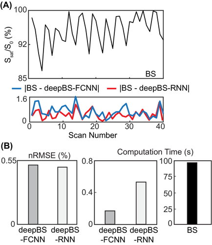
The performance of the deep Bloch simulators was benchmarked against ground-truth values from Bloch simulations, as shown in Figure 2. The residual error signals were calculated by subtracting the ground-truth MRF profiles from the MRF profiles estimated from the deep Bloch simulators (Figure 2A, bottom). The MTC-MRF profiles from the deep Bloch simulators agreed with the ground truths; however, the deepBS-RNN showed slightly higher accuracy than the deepBS-FCNN. The RMSE between the MRF profiles estimated from the deep Bloch simulators and the ground truths were 0.51% for deepBS-RNN versus 0.53% for deepBS-FCNN (Figure 2B). Importantly, the deep Bloch simulators achieved significantly higher computation efficiency (by a factor of ˜181 for deepBS-RNN and ˜570 for deepBS-FCNN) than the conventional Bloch simulation. Although the deepBS-RNN was slower than deepBS-FCNN (0.53 vs. 0.17 s), both Bloch simulators required less than a second for the prediction of a 10-k test data set and were computationally efficient, compared with the conventional Bloch simulation (96 s). Therefore, the slightly more accurate deepBS-RNN method was further used in the reconstruction framework.

4.2 Evaluation of reconstruction methods

The deep-learning MTC-MRF reconstruction methods were evaluated and validated using the numerical phantoms constructed by a two-pool Bloch simulation with a pseudo-randomized MRF schedule (Figure 3A). The Recon-RNN was compared with the Recon-FCNN to evaluate the reconstruction accuracy under various SNR levels to demonstrate generalization performance with respect to noise levels. The proposed Recon-RNN method outperformed the existing Recon-FCNN method in tissue-parameter quantification in terms robustness to noise (Figure 3B). In addition, the Recon-RNN outperformed dictionary-matching approaches (Figure S2A) in terms of reconstruction accuracy and computational speed. The higher-performing Recon-RNN was further trained and tested to estimate the MTC asymmetric effect. The nRMSE values of the Recon-RNN for the asymmetric MTC effect were 8.5% for k_mw, 3.1% for F, 1.5% for ${T}_2^{\mathrm{m}}$ , 1.1% for ${T}_1^{\mathrm{w}}$ , 3.4% for ∆_mw at an SNR of 46 dB. Figure 3C shows the cross-liked BSA phantom results. A variable RF saturation and acquisition schedule generated unique MTC signal profiles for the three compartments with different BSA concentrations.

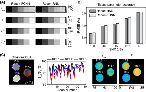
The Recon-RNN-based estimated pool size ratio was proportional to the known BSA concentration (10.5 ± 1.4% for 10% BSA, 17.8 ± 2.0% for 15% BSA, and 20.5 ± 1.9% for 20% BSA). However, the estimated value is not necessarily equal to BSA concentration, since it depends on how many macromolecular protons are present and participate in MT process with water.⁵⁴ Similar exchange rate values (109.9 ± 2.7 Hz for 10% BSA, 117.6 ± 3.8 Hz for 15% BSA, and 114.1 ± 5.1 Hz for 20% BSA) were estimated at constant pH 7.3.

4.3 In vivo MRI experiments

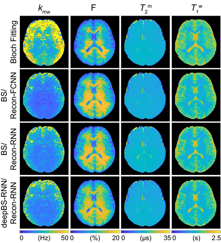
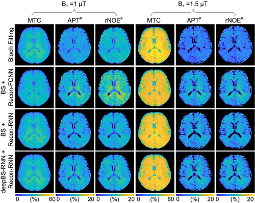
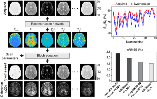
The Bloch simulator-driven, deep-learning reconstruction models were applied to the brains of healthy volunteers. Quantitative water and MTC parameter maps were successfully obtained in vivo using the conventional Bloch fitting, the deep-learning reconstruction models trained with two-pool Bloch simulations (BS/Recon-FCNN and BS/Recon-RNN), and the deep-learning reconstruction trained with the deep Bloch simulators (deepBS-RNN/Recon-RNN) as shown in Figure 4. In addition, the maps obtained from the deepBS-RNN/Recon-RNN method were compared with a conventional dictionary-matching approach (Figure S2B). The dictionary-matching method showed a poor reconstruction performance because of quantization errors from the discrete step size of the dictionary. The quantitative tissue-parameter maps generated from the BS/Recon-RNN method were in good agreement with the results obtained from the deepBS-RNN/Recon-RNN method (mean pSNR = 30.3 dB and mean SSIM = 0.96), but substantially reduced computation time for the generation of the training data set by about 181-fold (106 h for Bloch simulation and 35 min for the deepBS-RNN to generate a 40 million data set). The total reconstruction time of the Recon-RNN for an image matrix of 256 × 256 × 9 × 40 was 3 min 33 s, whereas the reconstruction time of the conventional Bloch fitting approach and dictionary matching (size = 200 k) approach was approximately 34 h and 19 min, respectively. In addition, APT^# and rNOE^# images were calculated by subtracting the saturated images at ±3.5 ppm from the symmetric (Δ_mw = 0) baseline reference images synthesized by solving a two-pool Bloch equation with estimated tissue parameters and scan parameters (Figure 5). Good agreement was found between the synthetic images generated from the RNN-based reconstruction models trained with Bloch simulation (BS/Recon-RNN) and the deep Bloch simulator (deepBS-RNN/Recon-RNN). The pSNR and SSIM values of the MTC, APT^#, and rNOE^# images between the BS/Recon-RNN and the deepBS-RNN/Recon-RNN were all above 40 dB and 0.96, respectively. However, the MTC signal intensity estimated from the Bloch fitting approach was slightly higher than that from the deep learning–based reconstruction methods, and, accordingly, lower APT^# and rNOE^# signal intensities were observed, particularly at 1.5 μT. Importantly, there were RF strength dependencies of the APT^# and rNOE^# signal intensities. At relatively low B₁ (1 μT), the upfield rNOE^# signal became more pronounced, compared with the downfield APT^# signal. Table 1 summarizes the averaged tissue parameters, MTC, APT^#, and rNOE^# for gray-matter and white-matter regions, estimated from the RNN-based MRF reconstruction with symmetric MTC assumption (Δ_mw = 0) (see also Table S1 for results from Bloch fitting, BS/Recon-FCNN, BS/Recon-RNN, and deepBS/Recon-RNN methods). These tissue parameters and MTC, APT^#, and rNOE^# signals were significantly different between white matter and gray matter (p < 0.05), except for ${T}_2^{\mathrm{m}}$ . For quantitative performance comparison in in vivo MRF images were synthesized with tissue parameters estimated from the different reconstruction methods and compared with experimentally acquired images, as shown in Figure 6. The mean nRMSE values for the deepBS-FCNN/Recon-FCNN, BS/Recon-FCNN, deepBS-RNN/Recon-RNN, and BS/Recon-RNN were 2.4%, 2.0%, 1.7%, and 1.5%, respectively. The Recon-RNN overall outperformed the Recon-FCNN method, which is consistent with the numerical phantom result.

TABLE 1. Estimated semisolid magnetization transfer contrast (MTC) parameters, free bulk water T₁ relaxation time, MTC at ±3.5 ppm, amide proton transfer (APT^#), and relayed nuclear Overhauser enhancement (rNOE^#) signal intensities (mean ± SD and 95% confidence interval) obtained from reconstruction with recurrent neural network (Recon-RNN) for white matter and gray matter of 8 healthy volunteer human brains.

ROIs		k_mw (Hz)	F (%)	T₂^m (μs)	T₁^w (s)	MTC(%)	APT^#(%)	rNOE^# (%)	MTC(%)	APT^#(%)	rNOE^# (%)
		k_mw (Hz)	F (%)	T₂^m (μs)	T₁^w (s)	B₁ = 1 μT			B₁ = 1.5 μT
WM	Mean ± STD	14.6 ± 0.9	17.0 ± 0.6	14.6 ± 0.5	1.1 ± 0.1	35.6 ± 0.4	9.5 ± 0.5	11.7 ± 0.5	51.8 ± 0.5	9.0 ± 0.7	9.3 ± 0.6
WM	95% CI	14.1 – 15.1	16.7 – 17.3	14.4 – 14.9	1.1 – 1.2	35.4 – 35.8	9.2 – 9.8	11.4 – 12.0	51.5 – 52.0	8.6 – 9.4	8.9 – 9.6
GM	Mean ± STD	19.8 ± 3.0	12.1 ± 1.3	14.9 ± 0.6	1.3 ± 0.1	32.9 ± 0.9	7.3 ± 0.9	9.3 ± 0.9	49.5 ± 1.2	6.1 ± 1.0	6.3 ± 1.1
GM	95% CI	18.2 – 21.5	11.4 – 12.9	14.5 – 15.2	1.2 – 1.4	32.4 – 33.4	6.9 – 7.8	8.8 – 9.7	48.8 – 50.1	5.6 – 6.6	5.7 – 6.9
p -value		< 0.01	< 0.01	0.24	< 0.01	< 0.01	< 0.01	< 0.01	< 0.01	< 0.01	< 0.01

Note: The Recon-RNN was trained with a 40 million data set synthesized from the RNN-based deep Bloch simulator (deepBS-RNN). Mean and SD values were obtained across subjects.
Abbreviations: CI, confidence interval; GM, gray matter; ROI, region of interest.

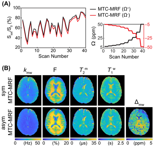
To evaluate the asymmetric MTC effect, MTC-MRF signal profiles were acquired at both positive frequency offsets (Ω⁺) and negative frequency offsets (Ω⁻), 80 dynamic scans in total. To display the MTC asymmetry effect, the MTC-MRF profile obtained from the negative frequency offsets was mirrored to the MTC-MRF profile from the positive frequency offsets, as shown in Figure 7A. Although most of the MTC-MRF (Ω⁻) signal intensities were lower than the MTC-MRF (Ω⁺) due to asymmetric MTC effects around the water resonance frequency, some signal intensities were quite similar at certain scan numbers because the asymmetric effect is dependent on the frequency offset and other scan parameters, such as saturation B₁ strength levels and durations. Figure 7B shows tissue-parameter maps estimated from the RNN-based reconstruction with only MTC-MRF (Ω⁺) and with both MTC-MRF (Ω⁺) and (Ω⁻). Note that the asymmetric tissue parameter maps (asym MTC-MRF) were reconstructed from 40 MTC-MRF (Ω⁺) and 40 MTC-MRF (Ω⁻) images (80 dynamic scans in total), whereas the symmetric tissue-parameter maps (symMTC-MRF) were reconstructed from only 40 MTC-MRF (Ω⁺) images. The chemical shift center (Δ_mw) was found to be 2.8 ± 0.1 ppm and 2.6 ± 0.2 ppm for the white matter and gray matter, respectively.

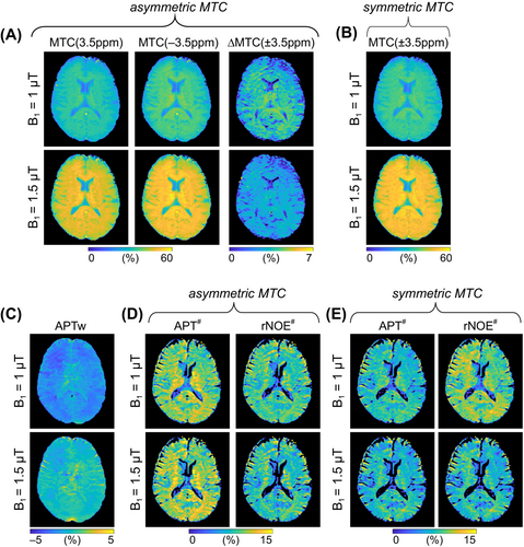
To investigate the asymmetric MTC effect on APT^# and rNOE^# images, asymmetric MTC images were synthetized using the tissue estimates from RNN-based reconstruction and scan parameters identical to those acquired in saturation images at ±3.5 ppm for APT^# and rNOE^# image calculation. The synthetic MTC images at ±3.5 ppm were generated with an assumption of asymmetric (Figure 8A) and symmetric (Figure 8B) MTC effects at RF saturation field strengths of 1 and 1.5 μT, respectively. With the assumption of the MTC asymmetry effect, overall MTC effects became more pronounced, which influenced APT^# and rNOE^# image contrast, as shown in Figure 8D,E. Several important results were observed: (i) The rNOE^# signal intensities with the asymmetric MTC effect were significantly lower than those with the symmetric MTC effect at 1 μT (p < 0.05) because the background baseline level (Z_ref = 100%−MTC) was lower when the asymmetric MTC component was added (see also Table S2); (ii) the broad MTC asymmetry also influenced downfield APT^# signal intensities (the APT^# signal intensities with the asymmetric MTC effect were higher than those with the symmetric MTC effects at the two RF saturation strength levels [p < 0.05] because the asymmetric super-Lorentzian lineshape signals spilled over into downfield frequency offsets from the water [Figure S3]); and (iii) at 1 μT, the APTw signal intensities were all negative (−2.1 ± 0.2% for white matter and −1.9 ± 0.3% for gray matter) due to a large upfield rNOE^#, whereas the APTw effect (−0.2 ± 0.3% for white matter and −0.3 ± 0.3% for gray matter) was more pronounced at 1.5 μT due to decreased rNOE^# and/or asymmetric MTC effects.

The repeatability of measurements by all reconstruction methods was evaluated by the test–retest study (Table 2). The within-subject CoV values for the deep-learning MRF reconstruction methods were less than 7% for all water and semisolid MTC parameters, and less than 10% for MTC, APT^#, and rNOE^# signals, indicating a high test–retest repeatability. The between-subject CoV values are reported in Table S3. The ICC values for test–retest reliability are presented in Table S4. An overall moderate reliability (ICC > 0.6) of the measurements was obtained.

TABLE 2. Within-subject coefficient of variance (CoV) of the estimated semisolid magnetization transfer contrast (MTC) parameters, free bulk water T₁ relaxation time, MTC at ±3.5 ppm, amide proton transfer (APT^#), and relayed nuclear Overhauser enhancement (rNOE^#) signal intensities obtained from Bloch fitting, Bloch simulation (BS)/reconstruction with fully connected neural network (Recon-FCNN), BS/reconstruction with recurrent neural network (Recon-RNN), and deep Bloch simulation (deepBS)/Recon-RNN methods.

Method	ROI	k_mw	F	${T}_2^{\mathrm{m}}$	${T}_1^{\mathrm{w}}$	MTC	APT^#	rNOE^#	MTC	APT^#	rNOE^#
		Coefficient of Variance
		k_mw	F	${T}_2^{\mathrm{m}}$	${T}_1^{\mathrm{w}}$	B₁ = 1 μT			B₁ = 1.5 μT
Bloch fitting	WM	4.3%	3.2%	0.7%	3.2%	0.5%	2.9%	2.4%	0.3%	4.9%	4.2%
Bloch fitting	GM	5.8%	2.7%	1.2%	2.0%	1.0%	4.1%	2.9%	0.8%	5.8%	6.9%
BS/Recon-FCNN	WM	2.1%	1.1%	1.0%	2.1%	0.8%	1.8%	1.7%	0.7%	2.9%	2.8%
BS/Recon-FCNN	GM	5.3%	3.4%	1.3%	3.0%	1.2%	2.7%	2.4%	1.3%	3.0%	3.7%
BS/Recon-RNN	WM	2.5%	1.4%	0.8%	2.1%	0.7%	3.0%	2.5%	0.6%	4.8%	4.2%
BS/Recon-RNN	GM	4.8%	3.7%	1.6%	3.1%	1.2%	4.3%	3.3%	1.1%	5.9%	6.9%
deepBS/Recon-RNN	WM	4.2%	1.4%	1.1%	1.6%	0.5%	2.7%	2.1%	0.5%	4.1%	3.0%
deepBS/Recon-RNN	GM	6.3%	3.5%	1.8%	3.8%	1.3%	5.0%	4.2%	1.4%	8.4%	9.1%

5 DISCUSSION

High-resolution MRF that includes a multipool exchange model requires an extremely large dictionary or training data set simulated with Bloch equations.^{40, 55} Furthermore, intensive Bloch simulation tasks are inevitable for MRF schedule optimization.^{44, 56} In this study, we developed a deep learning–based Bloch simulator for ultrafast MRF dictionary or training data generation, and a RNN for semisolid macromolecular MTC-MRF reconstruction. For MRF training data set generation, the deep Bloch simulator achieved a 181-fold reduction of the computation time compared with a conventional Bloch simulation. For MRF reconstruction, the deep-learning neural networks significantly reduced the reconstruction time without compromising reconstruction accuracy, approximate 570-fold reduction, compared with a Bloch equation–fitting approach without parallel computing. The proposed MRF reconstruction using RNNs outperformed the existing reconstruction methods, such as fully connected neural networks, Bloch fitting, and dictionary-matching methods in terms of tissue-parameter quantification accuracy. Importantly, the unified deep-learning framework, including an ultrafast Bloch simulator and MRF reconstruction, provided a high degree of repeatability.

The deep Bloch simulator mimics a conventional Bloch simulation to generate dictionaries or training data sets for MRF reconstruction more efficiently. For the semisolid MTC pool, a super-Lorentzian lineshape was used. The super-Lorentzian lineshape model includes an integration term to consider all possible dipolar orientations, requiring intensive computation. However, the deep Bloch simulator was able to address this computational challenge. For example, the deep Bloch simulator took only 34 min to generate 40 million training data sets for MRF RNNs, while the conventional Bloch simulation took about 107 h. In addition, the deep Bloch simulator substantially reduced the training time for MRF RNNs. During training of the reconstruction network (Figure 1C), the baseline MTC signal (Z_ref) was calculated for the loss function per iteration. For training the reconstruction network, the reconstruction network with the deep Bloch simulator took about 70 min for each epoch (1000 iterations), whereas the reconstruction network with the conventional Bloch simulation took about 4 days for each epoch and would take 6 months for 40 epochs. Furthermore, the deep Bloch simulator could be used to solve MRF-sequence optimization problems. In MRF sequence optimization, a very large number of MRF signal profiles must be simulated with updated tissue and scan parameters for each optimization iteration, which is computationally intensive.³⁷ The Bloch simulator needs to be retrained repeatedly for each MRF schedule tested, requiring intensive computation (about 27 h per epoch, including training data set generation and neural network training). However, the retraining of the Bloch simulator after each epoch during MRF optimization could be avoided if the RNN-based Bloch simulator is trained with various tissue parameters and scan parameters using a recently developed Only-Train-Once MRF (OTOM) method.^{57, 58} The current deep Bloch simulator can be trained with a fixed duration of the MRF sequence (e.g., 40 dynamic scans), which is a limitation in the optimization of the number of dynamic scans for acquisition efficiency. However, the RNN-based OTOM framework can be trained only once and applied to different types of MRF schedule with various schedule lengths. Therefore, combining the deep Bloch simulator with the OTOM method can improve the generalization ability and optimize the number of dynamic scans, improving scan efficiency. For the evaluation of MTC asymmetry in vivo, for the sake of simplicity, positive and negative frequency offsets were symmetrically acquired, instead of fully mixing frequency offsets. These frequency offsets need to be chosen to improve quantification accuracy of the chemical shift center of the semisolid macromolecular proton pool.

Regarding the accuracy of the deep Bloch simulator, errors may propagate into the subsequent MRF reconstruction network during the training process and lead to a difference in final tissue parameter maps. However, it was observed that the RMSEs were only 0.51% and 0.53% for deepBS-FCNN and deepBS-RNN, respectively, which are equivalent to the acquisition noise level (RMSE of 0.42% at SNR = 46 dB). In addition, through the Monte Carlo simulation study and the comparison study between BS-driven and deepBS-driven MRF reconstruction, the RNNs were demonstrated to be robust to noise and errors introduced from the deep Bloch simulators. In some cases, different parameter values were found between different methods (e.g., Bloch fitting vs. neural network–based reconstruction or Recon-FCNN vs. Recon-RNN), which may cause concern for disease evaluation. However, the signal difference from the different methods would not affect detection of disease-related contrast as long as consistent methodology is used when comparing healthy subjects with patients. In future work, the diagnostic accuracy of the deep learning methods to identify pathology will be evaluated.

The proposed Recon-RNN framework is based on a hybrid network architecture in which the input RNN layers enable an understanding of the temporal behavior of MTC-MRF profiles, the intermediate CNN layer extracts important features from each MRF profile in the temporal domain, and the last fully connected dense layers comply the features from the previous CNN layers to form the final output.^59-61 The hybrid architecture increased the reconstruction accuracy compared with the single FCNN model, whereas the reconstruction times were slightly longer, primarily because of the rectified linear unit activation functions used in BiLSTM, which is not currently supported by Computer Unified Device Architecture in TensorFlow environment (˜3.5 min for Recon-RNN vs. 11 s for Recon-FCNN vs. ˜34 h for Bloch equation fitting without parallel computing, for an image matrix of 256 × 256 × 9 × 40). Nevertheless, highly accurate and precise measurement of the semisolid MTC exchange rate is a very difficult task, as described previously,^{39, 40, 44} because the contribution of the MTC exchange rate to MR signals is very small and vulnerable to noise. Rather than improving the sensitivity and specificity of the exchange-rate estimation in the reconstruction process, the development of proton exchange–sensitizing RF labeling strategies may be rather desirable.^62-65 Using symmetric MTC, our estimated APT^# and rNOE^# signal intensities were slightly higher than the values reported previously,³⁴ likely due to differences in RF saturation parameters and direct water saturation effect. The previous study acquired MTC data with a fixed B₁ field strength of 2 μT and a saturation duration of 800 ms.

Several previous studies assumed a symmetric semisolid MTC effect because the semisolid macromolecular protons have a very broad RF absorption lineshape.^{13, 40, 56, 66} However, the MTC is caused by aliphatic protons, and experimental data have shown clear asymmetry around the water resonance.³¹ When using asymmetry in the MTC background, a higher pool size ratio of white matter is estimated (Figure 7B). Correspondingly, the MTC signal intensities at −3.5 ppm with asymmetric MTC were significantly higher than those with symmetric MTC, resulting in decreased rNOE^# signal intensities. With the inclusion of an asymmetric MTC, the semisolid macromolecular proton pool had a chemical shift center about 2.8 ppm upfield from the water resonance for white matter, which is consistent with the results (˜2.34 ppm for normal white matter) presented by Hua et al.³¹ Regarding the super-Lorentzian lineshape, the on-resonance singularity was handled by extrapolating gm(∆ω) from 1-kHz cut-off frequency to the asymptotic limit ∆ω → 0.^{13, 47} However, the choice of the cut-off frequency may affect MTC signal estimation, particularly at −3.5 ppm, because the frequency offset of rNOE is very close to the chemical shift center (∆_mw) of the semisolid macromolecular proton pool, as shown in Figure S3. Alternatively, the singularity could be avoided by integrating power spectral density of RF pulse over frequencies.⁶⁷

Along with quantification accuracy, the repeatability of the measurement plays a vital role in establishing an imaging method suitable for a clinical study. The test–retest repeatability from the CoV analysis was excellent for all tissue parameters, MTC, APT^#, and rNOE^# signals estimated from the deep Bloch simulator–driven MTC-MRF framework.

6 CONCLUSIONS

We developed a deep learning–based Bloch simulator for the ultrafast generation of MRF training data sets and a RNN for semisolid macromolecular MTC-MRF reconstruction. The deep Bloch simulator significantly reduced the computation time for the generation of training data sets compared with a conventional Bloch simulation. The RNN-based MRF reconstruction demonstrated advantages in terms of tissue-parameter quantification accuracy and computation efficiency. The test–retest study showed a high degree of repeatability of the proposed MTC-MRF framework in the brain and holds promise for assessing multiple tissue parameters simultaneously in a single scan.

ACKNOWLEDGMENTS

This work was supported, in part, by grants from the National Institutes of Health (R01EB029974, R01NS112242, R01AG069179, and P41EB031771).

CONFLICT OF INTEREST

Under a license agreement between Philips and the Johns Hopkins University, Dr. van Zijl, Dr. Zhou, and the University are entitled to fees related to an imaging device used in the study discussed in this publication. Dr. van Zijl is also a paid lecturer for Philips and receives research support from Philips. This arrangement has been reviewed and approved by the Johns Hopkins University in accordance with its conflict of interest policies.

Open Research

DATA AVAILABILITY STATEMENT

The source code is available at https://github.com/Heo-Group/DeepBS-MRF.

Supporting Information

Filename

Description

mrm29748-sup-0001-SupInfo.pdfPDF document, 1 MB

Figure S1. Regions of interest (ROIs) were drawn on T₂-weighted (T_2w) images. Eight subjects (S1–S8) participated in the test–retest study, whereas 3 subjects (S9–S11) participated in the magnetization transfer contrast (MTC) asymmetry study. T₂ maps are shown as references.

Figure S2. Comparison of the deep Bloch simulator (deepBS)–recurrent neural network (RNN)/reconstruction network using RNN (Recon-RNN) with the dictionary-matching method. (A) Bloch equation–based numerical phantom results. The normalized RMS error (nRMSE) values of the dictionary-matching method were 18.9% for k_mw, 6.2% for F, 2.5% for ${T}_2^{\mathrm{m}}$ , and 3.4% for ${T}_1^{\mathrm{w}}$ , whereas nRMSE values of the Recon-RNN were 9.1% for k_mw, 2.4% for F, 1.1% for ${T}_2^{\mathrm{m}}$ , and 0.8% for ${T}_1^{\mathrm{w}}$ . (B) In vivo tissue-parameter maps of a healthy volunteer brain. Note that the reconstruction accuracy of the dictionary-matching approach depends directly on the resolution of the dictionary (size = 200 k).

Figure S3. Semisolid absorption lineshapes (Lorentzian and super-Lorentzian) with/without magnetization transfer contrast (MTC) asymmetry (e.g., ∆_mw = 3 ppm). The super-Lorentzian functions are extrapolated from two cut-off frequencies (ε = 1 vs. 2 kHz) to model the semisolid macromolecular pool lineshape during on-resonance RF irradiation because the super-Lorentzian absorption lineshape has an on-resonance singularity (at ∆w = 0). With an asymmetric MTC, the lineshape center is shifted upfield from the water resonance; thus, the amplitude of the lineshape is increased at upfield frequency offsets but decreased at downfield frequency offsets (black vs. red for super-Lorentzian or green vs. blue for Lorentzian). Consequently, the shift can affect the overall MTC (or Z_ref), amide proton transfer (APT^#), and nuclear Overhauser enhancement (NOE^#) signal intensities.

Table S1. Estimated semisolid MTC parameters, free bulk water T₁ relaxation time, magnetization transfer contrast (MTC) at ±3.5 ppm, amide proton transfer (APT^#), and relayed nuclear Overhauser enhancement (rNOE^#) signal intensities (mean ± SD and 95% confidence interval) obtained from Bloch fitting, Bloch simulator (BS)/fully connected neural network (Recon-FCNN), BS/reconstruction network using RNN (Recon-RNN), and dense layers for the Bloch simulator (deepBS)–RNN/Recon-RNN methods for white matter and gray matter of the human brain. Mean and SD values were obtained across 8 subjects participated in test–retest study.

Table S2. Effect of symmetric versus asymmetric magnetization transfer contrast (MTC) on semisolid MTC parameters, free bulk-water T₁ relaxation time, MTC at +3.5 ppm, amide proton transfer (APT^#), and relayed nuclear Overhauser enhancement (rNOE^#) signal intensities (mean ± SD) in white matter and gray matter of the healthy volunteer human brain. All quantitative tissue parameters and signal intensities were estimated using reconstruction network using recurrent neural network (Recon-RNN). Mean and SD values were obtained across 3 subjects who participated in the study of asymmetric analysis.

Table S3. Between-subject coefficient of variance (CoV) of the estimated semisolid magnetization transfer contrast (MTC) parameters, free bulk-water T₁ relaxation time, MTC at ±3.5 ppm, amide proton transfer (APT^#), and relayed nuclear Overhauser enhancement (rNOE^#) signal intensities obtained from Bloch fitting, reconstruction network using fully connected neural network (Recon-FCNN), and reconstruction network using recurrent neural network (Recon-RNN) methods.

Table S4. Intraclass correlation coefficient (ICC) of the estimated semisolid magnetization transfer contrast (MTC) parameters, free bulk-water T₁ relaxation time, MTC at ±3.5 ppm, amide proton transfer (APT^#), and relayed nuclear Overhauser enhancement (rNOE^#) signal intensities obtained from Bloch fitting, Block simulation (BS)/reconstruction network using fully connected neural network (Recon-FCNN), BS/reconstruction network using recurrent neural network (Recon-RNN), and dense layers for the Bloch simulator (deepBS)–RNN/Recon-RNN methods. Mean ICC values were 0.6 ± 0.3, 0.6 ± 0.3, 0.6 ± 0.2, and 0.6 ± 0.1, corresponding to Bloch fitting, BS/Recon-FCNN, BS/Recon-RNN, and deepBS-RNN/Recon-RNN, respectively.

Please note: The publisher is not responsible for the content or functionality of any supporting information supplied by the authors. Any queries (other than missing content) should be directed to the corresponding author for the article.

REFERENCES

1Ward KM, Aletras AH, Balaban RS. A new class of contrast agents for MRI based on proton chemical exchange dependent saturation transfer (CEST). J Magn Reson. 2000; 143: 79-87.
10.1006/jmre.1999.1956
CAS PubMed Web of Science® Google Scholar
2Wolff SD, Balaban RS. Magnetization transfer contrast (MTC) and tissue water proton relaxation in vivo. Magn Reson Med. 1989; 10: 135-144.
10.1002/mrm.1910100113
CAS PubMed Web of Science® Google Scholar
3Henkelman RM, Huang X, Xiang QS, Stanisz GJ, Swanson SD, Bronskill MJ. Quantitative interpretation of magnetization transfer. Magn Reson Med. 1993; 29: 759-766.
10.1002/mrm.1910290607
CAS PubMed Web of Science® Google Scholar
4van Zijl PCM, Lam WW, Xu J, Knutsson L, Stanisz GJ. Magnetization transfer contrast and chemical exchange saturation transfer MRI. Features and analysis of the field-dependent saturation spectrum. Neuroimage. 2018; 168: 222-241.
10.1016/j.neuroimage.2017.04.045
PubMed Web of Science® Google Scholar
5Iannucci G, Rovaris M, Giacomotti L, Comi G, Filippi M. Correlation of multiple sclerosis measures derived from T₂-weighted, T₁-weighted, magnetization transfer, and diffusion tensor MR imaging. Am J Neuroradiol. 2001; 22: 1462-1467.
CAS PubMed Web of Science® Google Scholar
6Horsfield MA, Barker GJ, Barkhof F, Miller DH, Thompson AJ, Filippi M. Guidelines for using quantitative magnetization transfer magnetic resonance imaging for monitoring treatment of multiple sclerosis. J Magn Reson Imaging. 2003; 17: 389-397.
10.1002/jmri.10266
PubMed Web of Science® Google Scholar
7Sinson G, Bagley LJ, Cecil KM, et al. Magnetization transfer imaging and proton MR spectroscopy in the evaluation of axonal injury: correlation with clinical outcome after traumatic brain injury. Am J Neuroradiol. 2001; 22: 143-151.
CAS PubMed Web of Science® Google Scholar
8Cercignani M, Bozzali M, Iannucci G, Comi G, Filippi M. Magnetisation transfer ratio and mean diffusivity of normal appearing white and grey matter from patients with multiple sclerosis. J Neurol Neurosurg Psychiatry. 2001; 70: 311-317.
10.1136/jnnp.70.3.311
CAS PubMed Web of Science® Google Scholar
9Filippi M, Rocca MA, Rizzo G, et al. Magnetization transfer ratios in multiple sclerosis lesions enhancing after different doses of gadolinium. Neurology. 1998; 50: 1289-1293.
10.1212/WNL.50.5.1289
CAS PubMed Web of Science® Google Scholar
10Henkelman RM, Stanisz GJ, Graham SJ. A multicenter measurement of magnetization transfer ratio in normal white matter. J Magn Reson Imaging. 2000; 11: 568.
10.1002/(SICI)1522-2586(200005)11:5<568::AID-JMRI14>3.0.CO;2-8
CAS PubMed Web of Science® Google Scholar
11Morrison C, Stanisz G, Henkelman RM. Modeling magnetization transfer for biological-like systems using a semi-solid pool with a super-Lorentzian lineshape and dipolar reservoir. J Magn Reson B. 1995; 108: 103-113.
10.1006/jmrb.1995.1111
CAS PubMed Web of Science® Google Scholar
12Quesson B, Bouzier AK, Thiaudiere E, Delalande C, Merle M, Canioni P. Magnetization transfer fast imaging of implanted glioma in the rat brain at 4.7 T: interpretation using a binary spin-bath model. J Magn Reson Imaging. 1997; 7: 1076-1083.
10.1002/jmri.1880070621
CAS PubMed Web of Science® Google Scholar
13Heo HY, Zhang Y, Lee DH, Hong X, Zhou J. Quantitative assessment of amide proton transfer (APT) and nuclear overhauser enhancement (NOE) imaging with extrapolated semi-solid magnetization transfer reference (EMR) signals: application to a rat glioma model at 4.7 tesla. Magn Reson Med. 2016; 75: 137-149.
10.1002/mrm.25581
CAS PubMed Web of Science® Google Scholar
14Zhou J, Heo HY, Knutsson L, van Zijl PCM, Jiang S. APT-weighted MRI: techniques, current neuro applications, and challenging issues. J Magn Reson Imaging. 2019; 50: 347-364.
10.1002/jmri.26645
PubMed Web of Science® Google Scholar
15Heo HY, Zhang Y, Burton TM, et al. Improving the detection sensitivity of pH-weighted amide proton transfer MRI in acute stroke patients using extrapolated semisolid magnetization transfer reference signals. Magn Reson Med. 2017; 78: 871-880.
10.1002/mrm.26799
CAS PubMed Web of Science® Google Scholar
16van Zijl PCM, Yadav NN. Chemical exchange saturation transfer (CEST): what is in a name and what isn't? Magn Reson Med. 2011; 65: 927-948.
10.1002/mrm.22761
CAS PubMed Web of Science® Google Scholar
17Tee YK, Harston GW, Blockley N, et al. Comparing different analysis methods for quantifying the MRI amide proton transfer (APT) effect in hyperacute stroke patients. NMR Biomed. 2014; 27: 1019-1029.
10.1002/nbm.3147
CAS PubMed Web of Science® Google Scholar
18Sun PZ, Zhou J, Sun W, Huang J, van Zijl PCM. Detection of the ischemic penumbra using pH-weighted MRI. J Cereb Blood Flow Metab. 2007; 27: 1129-1136.
10.1038/sj.jcbfm.9600424
PubMed Web of Science® Google Scholar
19Heo HY, Tee YK, Harston G, Leigh R, Chappell MA. Amide proton transfer imaging in stroke. NMR Biomed. 2023; 36:e4734.
10.1002/nbm.4734
CAS PubMed Web of Science® Google Scholar
20Zhou J, Zaiss M, Knutsson L, et al. Review and consensus recommendations on clinical APT-weighted imaging approaches at 3T: application to brain tumors. Magn Reson Med. 2022; 88: 546-574.
10.1002/mrm.29241
PubMed Web of Science® Google Scholar
21Chen L, Wei Z, Chan KWY, et al. Protein aggregation linked to Alzheimer's disease revealed by saturation transfer MRI. Neuroimage. 2019; 188: 380-390.
10.1016/j.neuroimage.2018.12.018
CAS PubMed Web of Science® Google Scholar
22Jiang S, Eberhart CG, Lim M, et al. Identifying recurrent malignant glioma after treatment using amide proton transfer-weighted MR imaging: a validation study with image-guided stereotactic biopsy. Clin Cancer Res. 2019; 25: 552-561.
10.1158/1078-0432.CCR-18-1233
CAS PubMed Web of Science® Google Scholar
23Zaiss M, Windschuh J, Goerke S, et al. Downfield-NOE-suppressed amide-CEST-MRI at 7 Tesla provides a unique contrast in human glioblastoma. Magn Reson Med. 2017; 77: 196-208.
10.1002/mrm.26100
CAS PubMed Web of Science® Google Scholar
24Harston GW, Tee YK, Blockley N, et al. Identifying the ischaemic penumbra using pH-weighted magnetic resonance imaging. Brain. 2015; 138: 36-42.
10.1093/brain/awu374
PubMed Web of Science® Google Scholar
25Zu Z. Towards the complex dependence of MTRasym on T_1w in amide proton transfer (APT) imaging. NMR Biomed. 2018; 31:e3934.
10.1002/nbm.3934
PubMed Web of Science® Google Scholar
26Park JE, Kim HS, Park SY, Jung SC, Kim JH, Heo HY. Identification of early response to anti-angiogenic therapy in recurrent glioblastoma: amide proton transfer-weighted and perfusion-weighted MRI compared with diffusion-weighted MRI. Radiology. 2020; 295: 397-406.
10.1148/radiol.2020191376
PubMed Web of Science® Google Scholar
27Wen Q, Wang K, Hsu YC, et al. Chemical exchange saturation transfer imaging for epilepsy secondary to tuberous sclerosis complex at 3 T: optimization and analysis. NMR Biomed. 2021; 34:e4563.
10.1002/nbm.4563
CAS PubMed Web of Science® Google Scholar
28Zhou J, Payen J, Wilson DA, Traystman RJ, van Zijl PCM. Using the amide proton signals of intracellular proteins and peptides to detect pH effects in MRI. Nature Med. 2003; 9: 1085-1090.
10.1038/nm907
CAS PubMed Web of Science® Google Scholar
29Wang K, Wen Q, Wu D, et al. Lateralization of temporal lobe epileptic foci with automated chemical exchange saturation transfer measurements at 3 Tesla. EBioMedicine. 2023; 89:104460.
10.1016/j.ebiom.2023.104460
CAS PubMed Web of Science® Google Scholar
30Zhou J, Hong X, Zhao X, Gao JH, Yuan J. APT-weighted and NOE-weighted image contrasts in glioma with different RF saturation powers based on magnetization transfer ratio asymmetry analyses. Magn Reson Med. 2013; 70: 320-327.
10.1002/mrm.24784
CAS PubMed Web of Science® Google Scholar
31Hua J, Jones CK, Blakeley J, Smith SA, van Zijl PC, Zhou J. Quantitative description of the asymmetry in magnetization transfer effects around the water resonance in the human brain. Magn Reson Med. 2007; 58: 786-793.
10.1002/mrm.21387
CAS PubMed Web of Science® Google Scholar
32Paech D, Burth S, Windschuh J, et al. Nuclear Overhauser enhancement imaging of glioblastoma at 7 Tesla: region specific correlation with apparent diffusion coefficient and histology. PLoS One. 2015; 10:e0121220.
10.1371/journal.pone.0121220
PubMed Web of Science® Google Scholar
33Zhou Y, Bie C, van Zijl PCM, Yadav NN. The relayed nuclear overhauser effect in magnetization transfer and chemical exchange saturation transfer MRI. NMR Biomed. 2023; 36:e4778.
10.1002/nbm.4778
CAS PubMed Web of Science® Google Scholar
34Heo HY, Zhang Y, Jiang S, Lee DH, Zhou J. Quantitative assessment of amide proton transfer (APT) and nuclear overhauser enhancement (NOE) imaging with extrapolated semisolid magnetization transfer reference (EMR) signals: II. Comparison of three EMR models and application to human brain glioma at 3 Tesla. Magn Reson Med. 2016; 75: 1630-1639.
10.1002/mrm.25795
CAS PubMed Web of Science® Google Scholar
35Paech D, Zaiss M, Meissner JE, et al. Nuclear overhauser enhancement mediated chemical exchange saturation transfer imaging at 7 Tesla in glioblastoma patients. PLoS One. 2014; 9:e104181.
10.1371/journal.pone.0104181
PubMed Web of Science® Google Scholar
36Heo HY, Lee DH, Zhang Y, et al. Insight into the quantitative metrics of chemical exchange saturation transfer (CEST) imaging. Magn Reson Med. 2017; 77: 1853-1865.
10.1002/mrm.26264
CAS PubMed Web of Science® Google Scholar
37Perlman O, Farrar CT, Heo HY. MR fingerprinting for semisolid magnetization transfer and chemical exchange saturation transfer quantification. NMR Biomed. 2023; 36:e4710.
10.1002/nbm.4710
PubMed Web of Science® Google Scholar
38Ma D, Gulani V, Seiberlich N, et al. Magnetic resonance fingerprinting. Nature. 2013; 495: 187-192.
10.1038/nature11971
CAS PubMed Web of Science® Google Scholar
39Kang B, Kim B, Schar M, Park H, Heo HY. Unsupervised learning for magnetization transfer contrast MR fingerprinting: application to CEST and nuclear overhauser enhancement imaging. Magn Reson Med. 2021; 85: 2040-2054.
10.1002/mrm.28573
PubMed Web of Science® Google Scholar
40Kim B, Schar M, Park H, Heo HY. A deep learning approach for magnetization transfer contrast MR fingerprinting and chemical exchange saturation transfer imaging. Neuroimage. 2020; 221:117165.
10.1016/j.neuroimage.2020.117165
CAS PubMed Web of Science® Google Scholar
41Perlman O, Ito H, Herz K, et al. Quantitative imaging of apoptosis following oncolytic virotherapy by magnetic resonance fingerprinting aided by deep learning. Nat Biomed Eng. 2022; 6: 648-657.
10.1038/s41551-021-00809-7
CAS PubMed Web of Science® Google Scholar
42McGivney DF, Boyacioglu R, Jiang Y, et al. Magnetic resonance fingerprinting review part 2: technique and directions. J Magn Reson Imaging. 2020; 51: 993-1007.
10.1002/jmri.26877
PubMed Web of Science® Google Scholar
43Perlman O, Zhu B, Zaiss M, Rosen MS, Farrar CT. An end-to-end AI-based framework for automated discovery of rapid CEST/MT MRI acquisition protocols and molecular parameter quantification (AutoCEST). Magn Reson Med. 2022; 87: 2792-2810.
10.1002/mrm.29173
CAS PubMed Web of Science® Google Scholar
44Kang B, Kim B, Park H, Heo HY. Learning-based optimization of acquisition schedule for magnetization transfer contrast MR fingerprinting. NMR Biomed. 2022; 35:e4662.
10.1002/nbm.4662
PubMed Web of Science® Google Scholar
45Heo HY, Han Z, Jiang S, Schar M, van Zijl PCM, Zhou J. Quantifying amide proton exchange rate and concentration in chemical exchange saturation transfer imaging of the human brain. Neuroimage. 2019; 189: 202-213.
10.1016/j.neuroimage.2019.01.034
CAS PubMed Web of Science® Google Scholar
46Quesson B, Thiaudiere E, Delalande C, Chateil JF, Moonen CT, Canioni P. Magnetization transfer imaging of rat brain under non-steady-state conditions. Contrast prediction using a binary spin-bath model and a super-lorentzian lineshape. J Magn Reson. 1998; 130: 321-328.
10.1006/jmre.1997.1326
CAS PubMed Web of Science® Google Scholar
47Gloor M, Scheffler K, Bieri O. Quantitative magnetization transfer imaging using balanced SSFP. Magn Reson Med. 2008; 60: 691-700.
10.1002/mrm.21705
CAS PubMed Web of Science® Google Scholar
48Heo HY, Zhang Y, Jiang S, Zhou J. Influences of experimental parameters on chemical exchange saturation transfer (CEST) metrics of brain tumors using animal models at 4.7T. Magn Reson Med. 2019; 81: 316-330.
10.1002/mrm.27389
CAS PubMed Web of Science® Google Scholar
49Morrison C, Henkelman RM. A model for magnetization transfer in tissues. Magn Reson Med. 1995; 33: 475-482.
10.1002/mrm.1910330404
CAS PubMed Web of Science® Google Scholar
50Heo HY, Xu X, Jiang S, et al. Prospective acceleration of parallel RF transmission-based 3D chemical exchange saturation transfer imaging with compressed sensing. Magn Reson Med. 2019; 82: 1812-1821.
10.1002/mrm.27875
CAS PubMed Web of Science® Google Scholar
51Heo HY, Zhang Y, Lee DH, Jiang S, Zhao X, Zhou J. Accelerating chemical exchange saturation transfer (CEST) MRI by combining compressed sensing and sensitivity encoding techniques. Magn Reson Med. 2017; 77: 779-786.
10.1002/mrm.26141
CAS PubMed Web of Science® Google Scholar
52Kim M, Gillen J, Landman BA, Zhou J, van Zijl PC. Water saturation shift referencing (WASSR) for chemical exchange saturation transfer (CEST) experiments. Magn Reson Med. 2009; 61: 1441-1450.
10.1002/mrm.21873
CAS PubMed Web of Science® Google Scholar
53Kakite S, Dyvorne H, Besa C, et al. Hepatocellular carcinoma: short-term reproducibility of apparent diffusion coefficient and intravoxel incoherent motion parameters at 3.0T. J Magn Reson Imaging. 2015; 41: 149-156.
10.1002/jmri.24538
PubMed Web of Science® Google Scholar
54Malyarenko DI, Zimmermann EM, Adler J, Swanson SD. Magnetization transfer in lamellar liquid crystals. Magn Reson Med. 2014; 72: 1427-1434.
10.1002/mrm.25034
CAS PubMed Web of Science® Google Scholar
55Cohen O, Huang S, McMahon MT, Rosen MS, Farrar CT. Rapid and quantitative chemical exchange saturation transfer (CEST) imaging with magnetic resonance fingerprinting (MRF). Magn Reson Med. 2018; 80: 2449-2463.
10.1002/mrm.27221
CAS PubMed Web of Science® Google Scholar
56Perlman O, Herz K, Zaiss M, Cohen O, Rosen MS, Farrar CT. CEST MR-fingerprinting: practical considerations and insights for acquisition schedule design and improved reconstruction. Magn Reson Med. 2020; 83: 462-478.
10.1002/mrm.27937
PubMed Web of Science® Google Scholar
57Kang B, Heo HY, Park H. Only-train-once MR fingerprinting for magnetization transfer contrast quantification. Lect Notes Comput Sci. 2022; 13436: 387-396.
10.1007/978-3-031-16446-0_37
Google Scholar
58Kang B, Singh M, Park H, Heo HY. Only-train-once MR fingerprinting for B(0) and B(1) inhomogeneity correction in quantitative magnetization-transfer contrast. Magn Reson Med. 2023; 90: 90-102.
10.1002/mrm.29629
CAS PubMed Web of Science® Google Scholar
59Hopfield JJ. Neural networks and physical systems with emergent collective computational abilities. Proc Natl Acad Sci U S A. 1982; 79: 2554-2558.
10.1073/pnas.79.8.2554
CAS PubMed Web of Science® Google Scholar
60Schuster M, Paliwal KK. Bidirectional recurrent neural networks. IEEE Trans Signal Proces. 1997; 45: 2673-2681.
10.1109/78.650093
Web of Science® Google Scholar
61Alzubaidi L, Zhang J, Humaidi AJ, et al. Review of deep learning: concepts, CNN architectures, challenges, applications, future directions. J Big Data. 2021; 8: 53.
10.1186/s40537-021-00444-8
PubMed Web of Science® Google Scholar
62Knutsson L, Xu J, Ahlgren A, van Zijl PCM. CEST, ASL, and magnetization transfer contrast: how similar pulse sequences detect different phenomena. Magn Reson Med. 2018; 80: 1320-1340.
10.1002/mrm.27341
CAS PubMed Web of Science® Google Scholar
63Yadav NN, Jones CK, Hua J, Xu J, van Zijl PCM. Imaging of endogenous exchangeable proton signals in the human brain using frequency labeled exchange transfer imaging. Magn Reson Med. 2013; 69: 966-973.
10.1002/mrm.24655
CAS PubMed Web of Science® Google Scholar
64Zu Z, Xu J, Li H, et al. Imaging amide proton transfer and nuclear overhauser enhancement using chemical exchange rotation transfer (CERT). Magn Reson Med. 2014; 72: 471-476.
10.1002/mrm.24953
CAS PubMed Web of Science® Google Scholar
65Xu J, Yadav NN, Bar-Shir A, et al. Variable delay multi-pulse train for fast chemical exchange saturation transfer and relayed-nuclear overhauser enhancement MRI. Magn Reson Med. 2014; 71: 1798-1812.
10.1002/mrm.24850
CAS PubMed Web of Science® Google Scholar
66Lee DH, Heo HY, Zhang K, et al. Quantitative assessment of the effects of water proton concentration and water T₁ changes on amide proton transfer (APT) and nuclear overhauser enhancement (NOE) MRI: the origin of the APT imaging signal in brain tumor. Magn Reson Med. 2017; 77: 855-863.
10.1002/mrm.26131
CAS PubMed Web of Science® Google Scholar
67Asslander J, Gultekin C, Flassbeck S, Glaser SJ, Sodickson DK. Generalized Bloch model: a theory for pulsed magnetization transfer. Magn Reson Med. 2022; 87: 2003-2017.
10.1002/mrm.29071
CAS PubMed Web of Science® Google Scholar

Citing Literature

Volume90, Issue4

October 2023

Pages 1518-1536

This article also appears in:

Machine Learning and AI

Bloch simulator–driven deep recurrent neural network for magnetization transfer contrast MR fingerprinting and CEST imaging