The Importance of the Knowledge of Errors in the Measurements in the Determination of Copolymer Reactivity Ratios from Composition Data
Abstract
Often the errors in the measurement of copolymerizations are not accurately determined or included in the calculation of reactivity ratios. Some knowledge of the errors in the initial monomer ratio, conversion, and copolymer composition is however essential to obtain reliable (unbiased) reactivity ratios with a realistic uncertainty. It is shown that the errors serve a trifold purpose; they can serve as weighing factors in the fit, they can be compared with the fit residues to decide whether the chosen model is adequate for the data and they can be used to construct a realistic joint confidence interval for the reactivity ratios. The best approach is to have an estimate of the individual errors in the copolymer composition, either from a thorough error propagation exercise or from replicate measurements. With these errors, the χ2-joint confidence intervals can then be constructed which gives a realistic estimate of the errors in the reactivity ratios. Utilizing the Errors in Variables Method (EVM) is correct and useful, but only if the individual errors in all the variables in each experiment are more or less known.
1 Introduction
In this equation F1 is the fraction of monomer 1 in the copolymer, f1 is the (mole) fraction of monomer 1 in the (reacting) feed, and r1 is the ratio of propagation rate coefficients for chain-end 1 adding to monomers 1 and 2 and r2 for chain end 2 adding to monomers 2 and 1. Equation (1) makes clear that (instantaneous) copolymer composition does not depend on all four propagation rate coefficients individually, and similarly, it depends on monomer mole fractions rather than monomer concentrations. This equation is only for instantaneous (not cumulative) composition where f1 equals the initial monomer mole fraction f10, not affected by conversion (X). In deriving it assumes that chains are long (i.e., chain-starting and -stopping reactions have a negligible effect on overall composition) and that radical reactivity is determined only by the last unit of growing chains (the so-called terminal model). In 1952 the first book on copolymerization appeared.[2] O'Driscoll published a series of early papers on copolymerization between 1964 and 1969.[3-9] The pivotal paper of O'Driscoll was published in 1980 together with Randall McFarlane and Park Reilly.[10] Around that time the Eindhoven group started publishing on the correct determination of reactivity ratios as well.[11] Important contributions also came from the University of Waterloo where the errors in all variables method (EVM) were captured in the RREVM computer program.[12]
-
Use only non-linear regression (NLLS) or Visualization of the Sum of Squares Space methods (VSSS).[14, 15]
-
Either use low conversion f0-F data or conversion dependent data in the form of f0-f-X or f0-X-F, in all cases with at least three different starting monomer compositions f0.
-
Obtain the best possible information about the errors in the measurements, and utilize weighting according to the errors in the dependent variable (in most cases F).
-
If the independent variable (usually f) has considerable error, use EVM.
-
Be aware of errors in f0, especially in conversion dependent experiments.
-
Analyze the residuals and compare the fit residuals with the estimated errors.
-
The obtained reactivity ratios should be reported with the correct number of significant digits (typically 2) and a measure of the uncertainty in those values (preferably a joint confidence interval).
In this paper, we want to give special attention to the aspect of knowledge of the errors in the measurements, with respect to recommendations 3, 4, 5, 6, and 7. Points 1 and 2 mainly concern the data and the model but not its error structure.
1.1 Errors in the Measurements
First of all, we have to distinguish random errors from systematic errors. In the assumptions for non-linear regression, it is assumed that the errors in the measurements are independent and normally distributed (Gaussian distribution). Unfortunately, systematic errors cannot always be avoided.[13] In the IUPAC recommended method, the initial monomer fraction (f0) the molar conversion (X), and the copolymer composition (F) should be measured, the so-called f0-X-F method. For f0 typically the weight of the two monomers is used, which can be quite accurate. Then for the conversion often the mass conversion is converted to a molar conversion, alternatively, in Nuclear Magnetic Resonance (NMR) experiments, the conversion can be obtained from the partial conversions of both monomers. For the copolymer composition, a sample can be taken and analyzed with for, example, NMR[16], IR spectroscopy, or elemental analysis.[14] An often used method is to do a copolymerization experiment in an NMR tube and measure the conversion of the two monomers, the so-called f0-f-X method, and either fit these data directly or after converting f to F.[13]
1.2 Errors in f0
Most often f0 values are assumed to contain no error. In the NMR experiment, the f0 can either be used from gravimetry or as the value obtained by integration of the NMR signals at zero conversion (sometimes extrapolated back to zero conversion from later data). Although both values should be closely matched, slight differences might occur. It has been established that small changes in f0 have a major influence on the obtained reactivity ratios. The reason is that in the f0-f-X method, the calculations are always relative to the value of f0 and a small error already results in a systematic bias in the fit. This effect has previously remained unnoticed. Also for the method, similar issues with f0 can arise.[13]
In the IUPAC paper[13] this effect has been shown clearly in a X versus f dataset for X data with random noise. Here we show, for a different dataset with Gaussian noise, that when only changing the f10 value (introducing a systematic error in the data) the change in reactivity ratios is very large (Figure 1).
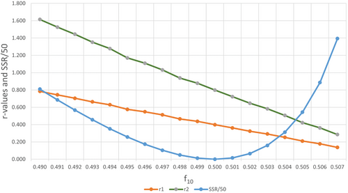
A change in f10 of −0.001 shifts r1 from 0.4 to 0.438 and r2 from 0.8 to 0.878. The typical random error in NMR for f10 is most likely already larger than 0.001 (data in Table S1, Supporting Information). This means that even with a very accurate value of f10 one might want to optimize this value. The errors in all variables method (RREVM) does not take these small errors in f10 into account.[12] Only recently some software[13, 17] has been equipped to test for these small variations in f10. Alternatively one can use hierarchical methods.[18]
The errors in the measurements of X, f, and F can be obtained either by a thorough error propagation exercise or by repeat experiments. These errors serve the purpose of weighing those data in the fit, determining whether the fit residuals are not larger than expected, and also determining the size of the Joint Confidence Intervals in the case of using the X2 method (see section on the joint confidence intervals).
Fitting without giving any information on the errors in the measurements is sometimes done (can be done for example in Excel). The problem is that the fit residues then are used to estimate the uncertainty in the parameters. With that approach, it is assumed that the model is correct. In a regular approach comparing the fit residues with the estimated errors is actually a means to determine whether the model is correct[15], so one loses this information if no error estimates are included in the fit. Furthermore, unbiased values for the reactivity ratios depend on the utilization of the errors in the measurements.
1.3 The Errors in all Variables Method
Already for a long time, researchers have agreed that the errors in all variables should be taken into account when fitting reactivity ratios. As early as 1978 Van der Meer, Linssen, and German introduced the errors in (both) variables method[1] (EVM). Many papers appeared since, of which a more recent description of the well-known software RREVM appeared in 2018.[12] Taking this last paper as the benchmark, there are a few remarks to be made. As EVM applied to low conversion f-F data takes the errors in both monomer fraction (f) and copolymer composition (F) into account, it seems that this should be the preferred method of dealing with the errors in both variables. These errors are used to calculate the approximate joint confidence intervals (JCI) based on the X2 distribution. However, if we read the 2018 paper carefully, it turns out that the user of the software might not actually pay much attention to the actual errors in the measurements:“ The program's default settings assume 1% error associated with feed composition and 5% error associated with cumulative copolymer composition.” Two issues with this approach; the error is taken as multiplicative, which is not the most likely error structure[13], furthermore switching the labels of the monomers while keeping the multiplicative errors the same, leads to different answers for reactivity ratios and joint confidence intervals as shown in the paper.[12, 13] Besides these two points, it is strange, to say the least, that EVM (in this case) implies to deal with errors in the measurements correctly, but actually does not really deal with individual errors in each measurement. The handwaving approach to just assume a constant percentual error over the whole range of data is in most cases not correct. Depending on how the data are measured, the absolute error might show a trend not matching a constant relative error (see for example ref 14 and example later) nor a constant absolute error.
As an example; a typical experiment to collect many data is to monitor the monomer conversions with NMR. The signal-to-noise ratio might change with conversion, decreasing at higher conversions. When the data are converted to copolymer compositions, the low conversion data have a large propagated error[13](at low conversion the shift in f is very small, leading to large errors in F). The individual errors per measurement should be used as weighing factors[15](see example later).
The question is now whether using EVM with handwaving the actual errors in the measurement is preferred over an approach where the actual errors are included in the calculations (maybe not even using EVM). Going back to the popular NMR experiments, with knowledge of the errors in f10, X, and f, through error propagation, a realistic error in the copolymer composition can be estimated. This error doesn't follow either a constant absolute or relative error (see SI of reference 13 and the example below).
1.4 Weighing of the Individual Experiments
Often the errors in the measurements are not really estimated and for that reason weighing the individual measurements with their error (a larger error leads to a smaller weight in the fit) is also omitted. Leaving out the weighing can lead to erroneous results in some cases. An example is where copolymer compositions are calculated from NMR data on the monomer consumption. At low conversions, the shift in f is very small leading to large errors in F. Through proper error propagation the errors in F can be calculated and should be used as weights. Here a dataset generated with Gaussian noise with a standard deviation of 0.01 on both conversion and monomer ratio is given, based on reactivity ratios of r1 = 0.4, r2 = 1.4:
| f10 | f | X | ΔX | Δf | F | ΔF |
|---|---|---|---|---|---|---|
| 0.5 | 0.5138 | 0.0684 | 0.005 | 0.005 | 0.3117 | 0.06972 |
| 0.5 | 0.5244 | 0.1383 | 0.005 | 0.005 | 0.3477 | 0.03181 |
| 0.5 | 0.5310 | 0.2024 | 0.005 | 0.005 | 0.3777 | 0.02007 |
| 0.5 | 0.6252 | 0.5999 | 0.005 | 0.005 | 0.4165 | 0.00376 |
| 0.5 | 0.7820 | 0.8557 | 0.005 | 0.007 | 0.4525 | 0.00226 |
| 0.5 | 0.9193 | 0.9536 | 0.005 | 0.01 | 0.4796 | 0.00236 |
| 0.5 | 0.9464 | 0.9703 | 0.005 | 0.01 | 0.4864 | 0.00239 |
| 0.7 | 0.7130 | 0.0600 | 0.005 | 0.005 | 0.4957 | 0.08044 |
| 0.7 | 0.7233 | 0.1186 | 0.005 | 0.005 | 0.5265 | 0.03807 |
| 0.7 | 0.7348 | 0.1761 | 0.005 | 0.005 | 0.5370 | 0.02406 |
| 0.7 | 0.8063 | 0.5213 | 0.005 | 0.005 | 0.6024 | 0.00499 |
| 0.7 | 0.8679 | 0.7041 | 0.005 | 0.005 | 0.6294 | 0.00270 |
| 0.7 | 0.8765 | 0.7291 | 0.005 | 0.007 | 0.6344 | 0.00309 |
| 0.7 | 0.9789 | 0.9412 | 0.005 | 0.01 | 0.6826 | 0.00169 |
| 0.9 | 0.9101 | 0.1008 | 0.005 | 0.005 | 0.8098 | 0.04488 |
| 0.9 | 0.9234 | 0.1940 | 0.005 | 0.005 | 0.8028 | 0.02100 |
| 0.9 | 0.9727 | 0.6438 | 0.005 | 0.005 | 0.8598 | 0.00290 |
| 0.9 | 0.9770 | 0.7314 | 0.005 | 0.007 | 0.8717 | 0.00267 |
| 0.9 | 0.9870 | 0.8360 | 0.005 | 0.009 | 0.8829 | 0.00187 |
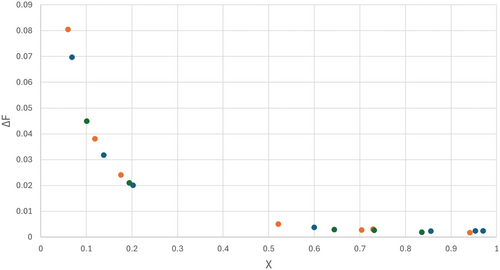
Shown in Figure 2, the errors in F after conversion of f to copolymer composition F, including error propagation to ΔF from the errors in f and X. The error in F ranges from 0.08 at low conversion to 0.002 at higher conversion (a factor of 40 in the weight of these data in the fit). Note that due to the direction of the composition drift, in this case the higher values of F have the lower ΔF values.
The values compare very well to the reactivity ratios that were used to generate the noisy data (r1 = 0.4, r2 = 1.4).
Applying this weighing scheme the fit gives answers further away from the true values and with much larger standard deviations. The standard deviations are calculated from the JCI (X2) and hold contributions from the (weighted) sum of squares of residuals at the minimum and the (weighted) estimated errors. In uniform weighting, all points carry the same weight and the estimated errors are not relevant, in this case giving the inaccurate low conversion data too much weight.
In case the copolymer compositions are measured directly (eg with NMR[16], infrared spectroscopy, elemental analysis[14] or otherwise) the error structure could look completely different from Figure 2. In NMR the peaks are sometimes partially overlapping and the signal-to-noise ratio changes with conversion, leading to errors in the copolymer composition that follow neither a constant absolute nor a constant relative error.[16]
1.5 The Shape and Size of the Joint Confidence Interval
As indicated it is necessary to use the individual errors as weighing factors in the fit and they can also be used to estimate the JCI with correct shape through the use of the visualization of the sum of squares space (VSSS) and the X2 distribution.[13]
Here σ2 corresponds to the average absolute variance of the dependent variable (in this case F) and is calculated from the well-estimated errors as entered by the user. ssmin(r1,r2) is the sum of squares of residuals at the minimum and with p degrees of freedom (p equals two in the present cases).
With this approach, it is not only the fit residuals that contribute to the size of the JCI, but also the estimated errors in the measurements. It would be most reassuring if the theoretical sum of squares of residuals (from estimated errors) is in the same order of magnitude as the actual sum of squares of residuals (from the fit).
In this approach the errors as estimated by the user do not play a role. If one has a good fit (ssmin(r1,r2) small) the JCI will be small, which can be a coincidence as illustrated below.
When the same series of experiments is repeated several times, due to the random errors in the data, the results for the JCI are different every time (see Figure 3). This variation in the end will be better reflected by taking into account the actual errors in the measurements than the fit residuals of one of such a series of experiments only.
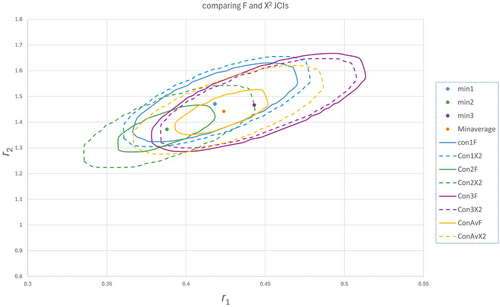
To illustrate this a set with 9 datapoints evenly distributed and with Gaussian noise with a standard deviation of 0.01 was generated based on reactivity ratios of 0.4 and 1.4 (Table S2a–c, Supporting Information). The reactivity ratios from three of those sets are shown in Figure 3, together with the JCIs based on the fit residuals combined with the Fisher distribution (called F-JCI, Equation (5)) as well as JCIs based on the fit residuals plus the estimated errors and the χ2 distribution (called χ2 -JCI, Equation (4), dotted lines).
Depending on the goodness of fit the F- and χ2- JCIs are similar (blue and purple) or in some cases, the F-JCI is much smaller than the one based on χ2 (green). As mentioned before, the size of the F-JCI depends mainly on the fit residuals whereas in the χ2 -JCI there is always the maximum contribution of the estimated errors in F. It is also clear that with a realistic standard deviation of 0.01 in F, the reactivity ratios vary a lot and some of the F-JCIs actually do not encapsulate the minimum of other sets. So it is advisable to do multiple experiments and average the F values so obtained. If we average the 3 sets, we get a new set (yellow) which seems closer to the real values and the fit is better, but the F-JCI seems too small and it is better to take the χ2-JCI with the errors properly estimated in order to also encapsulate r-values from the other sets and to give a reflection of the actual inaccuracy of the r-values.
It has to be noted that averaging of 3 datasets and generating a new dataset does not change the number of datapoints, but normally would result in new estimates of the standard deviations. In this simulated case the standard deviations are known and used to generate the gaussian noise and averaging does not change the standard deviation either (0.01). The main effect of averaging here is getting a better estimate of the reactivity ratios and in the F-approach (because of smaller fit residues) a smaller JCI. The JCI's for the χ2 approach are therefore all similar in size, including that of the averages. With experimental data, this might be slightly different as a better estimate of the standard deviation is obtained which will affect the size of the χ2 -JCI also.
Furthermore, the NLLS data from reference 13 were taken and a χ2-JCI (ESD 0.01) was generated from one of the datasets. 100 point estimates for the reactivity ratios were generated (Table S3, Supporting Information) with Gaussian noise and are shown in Figure 4a,b, together with the χ2-JCI. The χ2-JCI safely encapsulate almost all generated point estimates of r1 and r2. Often the F-JCIs are smaller and more variable, so therefore it is saver to use the χ2-JCI.
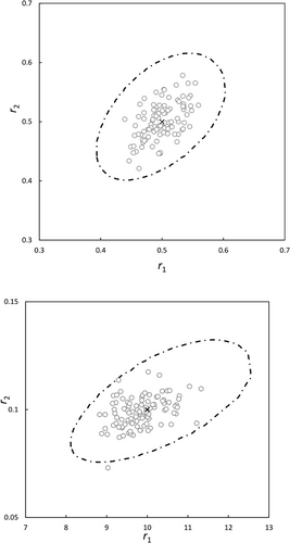
It must be mentioned here that by utilizing VSSS one obtains the JCIs with true shape which is not 100% symmetrical. Furthermore the sizes of the F-JCIs are varying substantially (less so the χ2-JCIs), depending on which of the sets with Gaussian noise is chosen, but the overall picture remains the same. In the authors experience the F-JCIs are often somewhat smaller than the χ2-JCIs.
2 Conclusion
Often the errors in the measurement of copolymerizations are not accurately determined and included in the calculation of reactivity ratios. It is shown that some knowledge of the errors in variables is essential to obtain reliable reactivity ratios with a realistic uncertainty (standard deviation).
The errors serve a trifold purpose; they must serve as weighing factors in the fit, they must be compared with the fit residues to decide on whether the chosen model is adequate for the data and they can be used to construct a realistic joint confidence interval for the reactivity ratios. Assuming a simple error structure in the data (constant relative error or constant absolute error) in most cases is not appropriate and can lead to wrong values of the reactivity ratios as well as over- or underestimation of their uncertainties. Utilizing the χ2-JCI is preferred over the F-JCIs because the latter are more variable and often underestimate the uncertainty.
The best approach is to have an estimate of the individual errors in the copolymer composition, either from a thorough error propagation exercise or from replicate measurements. With these errors, the χ2-JCI can then be constructed which gives a realistic estimate of the errors in the reactivity ratios.
Software that requires errors in the copolymer composition and can also investigate the influence of small variations in the initial monomer fractions has recently become available.[17]
Utilizing the Errors in Variables Method is correct and useful, but only if the individual errors in both f and F in each experiment are more or less known and utilized in the calculations, both in weighing and in determining the size of JCI.
Handwaving the error structure (utilizing constant relative or constant absolute error for all data) while utilizing EVM gives a false sense of accuracy of the obtained reactivity ratios.
Acknowledgements
The author would like to acknowledge Dr Robert Reischke (Postdoctoral Fellow at AIfA Bonn) for valuable discussions and critically reading the manuscript.
Conflict of Interest
The authors declare no conflict of interest.
Open Research
Data Availability Statement
The data that support the findings of this study are available from the corresponding author upon reasonable request.


