Biomechanical evaluation of total ankle arthroplasty. Part I: Joint loads during simulated level walking
Abstract
In total ankle arthroplasty, the interaction at the joint between implant and bone is driven by a complex loading environment. Unfortunately, little is known about the loads at the ankle during daily activities since earlier attempts use two- or three-dimensional models to explore simplified joint mechanics. Our goal was to develop a framework to calculate multi-axial loads at the joint during simulated level walking following total ankle arthroplasty. To accomplish this, we combined robotic simulations of level walking at one-quarter bodyweight in three cadaveric foot and ankle specimens with musculoskeletal modeling to calculate the multi-axial forces and moments at the ankle during the stance phase. The peak compressive forces calculated were between 720 and 873 N occurring around 77%–80% of stance. The peak moment, which was the internal moment for all specimens, was between 6.1 and 11.6 N m and occurred between 72% and 88% of the stance phase. The peak moment did not necessarily occur with the peak force. The ankle joint loads calculated in this study correspond well to previous attempts in the literature; however, our robotic simulator and framework provide an opportunity to resolve the resultant three-dimensional forces and moments as others have not in previous studies. The framework may be useful to calculate ankle joint loads in cadaveric specimens as the first step in evaluating bone–implant interactions in total ankle replacement using specimen specific inputs. This approach also provides a unique opportunity to evaluate changes in joint loads and kinematics following surgical interventions of the foot and ankle.
1 INTRODUCTION
Aseptic loosening, osteolysis, and subsidence are among the most common complications of total ankle arthroplasty, occurring in approximately 15% to 30% of patients postoperatively.1-5 Although multi-factorial in nature, all three are directly related to the biomechanical interaction between the implant and bone.6 For example, excessive relative micromotion between the implant and the bone prevents bone ingrowth, which may result in early aseptic loosening.7 Excessive loads across the articulating surfaces can lead to increased polyethylene wear, which may lead to osteolysis.6 Similarly, improper load transfer between implant and bone can cause overloading of the bone, which may lead to subsidence of the components.6 Thus, the interaction between the implant and bone is driven by the complex loading environment at the ankle joint.
Unfortunately, although joint loading directly affects these complications, little is known about the loads at the ankle during daily activities. Early attempts to determine ankle loads used two- or three-dimensional models to explore simplified motions of the joint.8-10 Modern musculoskeletal models incorporated more physiological movements derived from skin motion marker data to predict muscle forces and resultant loads.11-13 These models provided useful information about the kinematics and ankle joint loads for in vivo subjects; however, the models often need to be simplified to predict muscle forces. All these models predict muscle forces that completely compensate for the joint torques caused by the external loads, resulting in scenarios with zero moments acting about the joint axes. Since the external loads and the ankle kinematics during activity are undoubtedly three-dimensional,11 these models do not account for all dimensions when determining loads of the internal structures. Therefore, model predictions that lack the contribution of resultant moments at the ankle joint do not entirely capture the complexity of the loading environment.
Finite element models have long been used in biomechanical studies to evaluate bone–implant interactions. However, for ankle arthroplasty, these models have considered one or, at best, a few loading cases. Often the worst-case loading scenario is assumed to occur at the instance of the peak compressive force, near toe-off.14-16 Conversely, studies in other joints like the knee, for which much more is known about the loading environment, have demonstrated the importance of considering multi-axial forces and moments when evaluating bone–implant interaction, where submaximal forces and high moments resulted in the peak burden at the interface.17, 18 Therefore, it is unclear whether the loading conditions considered in finite element studies of ankle replacements truly represent the worst-case scenario for the interaction between the implant and bone.
To address these shortcomings in the current understanding of the biomechanics of total ankle arthroplasty, we developed a framework that integrated robotic gait simulations of cadaveric specimens, musculoskeletal models, and finite element models to evaluate the interaction between the implant and bone. The overarching aims of our two-part study were (1) to determine the multi-axial loads at the joint during simulated level walking following total ankle arthroplasty and (2) to determine how the loads and the fixation design of the tibial component impact the interaction between the implant and the bone. In this first part of our two-part study, we describe how we combined our previously developed robotic gait simulator with musculoskeletal modeling to calculate the multi-axial forces and moments acting at the implanted ankle during the stance phase of simulated level walking. These loads were then used in Part II to drive finite element models to evaluate the interaction between the tibial component of a total ankle arthroplasty implant and the surrounding bone.
2 METHODS
Our framework to calculate ankle joint loads began by reproducing the stance phase of level walking using our robotic gait simulator in cadaveric foot and ankle specimens implanted with a total ankle replacement. Level walking was simulated by recreating the relative motion of a force plate with respect to the tibia and muscle activation from in vivo human subjects. The outputs collected from the robotic simulations were the individual bone kinematics, muscle-tendon forces, and ground reaction forces. The simulator outputs and bone morphology were then used to develop musculoskeletal models and calculate ankle joint loads specific to each specimen. In Part II, the calculated loads were then applied to finite element models developed using the tibial morphology and implant position to predict bone–implant micromotions and periprosthetic bone strains as measures of fixation.
2.1 Robotic gait simulation
Three male cadaveric foot-to-mid-tibia specimens with neutral foot alignment and no history of lower extremity trauma or surgery were used for the robotic simulations (Table 1). A board-certified orthopedic surgeon experienced in total ankle arthroplasty then implanted each specimen with a contemporary ankle replacement (INFINITY™, Wright Medical Group, Inc.) using specimen-specific PROPHECY™ INFINITY™ guides based on the manufacturer procedure and the incision was closed with sutures. The size of the commercial implants used were based on the expertise and experience of the board-certified orthopedic surgeon (CD). Clusters of four retro-reflective markers were rigidly fixed to the tibia and talus using intracortical bone pins to quantify joint kinematics during the subsequent robotic simulations. Skin and muscle were removed from 10 cm of the proximal tibia to be potted in poly-methyl methacrylate, the proximal Achilles tendon was secured to a linear actuator with an aluminum clamp, and the proximal ends to the eight smaller tendons were grasped with a clove hitch knot that was reinforced with a screw and nut to attach to the actuators, following a previously developed protocol.19 The remainder of the cadaveric specimen was left intact.
| Specimen | Side | Age | Sex | Height (cm) | Weight (kg) | BMI (kg/m2) | Foot length (mm) |
|---|---|---|---|---|---|---|---|
| S-1 | L | 51 | M | 185 | 104 | 30 | 235 |
| S-2 | L | 59 | M | 178 | 76 | 24 | 240 |
| S-3 | L | 61 | M | 183 | 71 | 21 | 245 |
Each specimen was tested on a robotic simulator that has been validated to reproduce in vivo foot and ankle kinematics (Figure 1).19 In brief, the simulator consists of a six-degree-of-freedom force plate and nine linear actuators for the intrinsic muscle-tendons of the foot and ankle. The simulator uses in vivo tibial motions and ground reaction forces collected from healthy adult males and muscle activation from electromyography as inputs to simulate level walking of healthy human subjects. An iterative control algorithm is then used to adjust the trajectory of the force plate and the forces of the Achilles and tibialis anterior tendons to reduce the error between the target and measured ground reaction forces. After the robot converges on a force plate trajectory that minimizes error in the ground reaction forces, an 8-camera motion capture system (T-40s, Vicon Motion Systems) is used to collect the motion of the marker clusters secured to the individual bones throughout the stance phase.

Simulations were conducted at one-sixth the average time of in vivo stance and at one-quarter bodyweight (3.6 s and 175 N, respectively). These conditions mitigated the risk of damaging the specimens and simulated loading representative of partial weight-bearing at the beginning of patient rehabilitation following total ankle arthroplasty. In addition to recording the motion capture results, the ground reaction forces and center of pressure from the force plate and the tendon forces from the nine linear actuators were collected throughout the stance phase. After stance simulations, the foot was loaded with a vertical ground reaction force of 100 N, and the tension applied to the Achilles tendon was set at 100 N to simulate a standing pose and define the neutral joint positions.
2.2 Kinematics
All outputs from the simulator were transformed into a coordinate system based on the baseplate of the tibial implant to report joint loads with respect to the implant. The implant coordinate system was defined by the anterior–posterior and medial–lateral directions of the device with the origin at the intersection on the bone–implant interface. The positions of the marker clusters during stance simulations with respect to standing were transformed into the implant coordinate system and then used to calculate the change in rotational kinematics. Translation of the talus implant with respect to the tibial implant was neglected since this translation was small given the constraint of the implant design. Contact between components was not simulated.
2.3 Ground reaction forces
During cadaveric gait simulations, the inertial loads are subtracted from the measured ground reaction forces, both of which are repeatable and have been discussed previously.19-21 For the musculoskeletal models, the raw inertial readings and the raw simulation readings for the ground reaction forces were collected from the robot and transformed into the implant coordinate system before subtracting. This provided the resultant ground reaction force and the corresponding center of pressure reported in the implant coordinates throughout the stance simulations.
Four retroreflective markers were attached to the force plate to record the plate movement with motion capture cameras throughout the stance trajectory. Before testing, a 3D coordinate digitizer with a standard error measurement of 0.018 mm (FARO Gage, FARO Technologies, Inc.) was used for digitizing locations of the marker centroids and the coefficients defining the planes of the force plate in the digitizer coordinate system. The markers and planes of the force plate were digitized in the ground position of the robot, where the force plate was parallel to the floor. The digitized coefficients of the top plane, the anterior–posterior planes, and the medial–lateral planes were used to approximate the origin of the force plate, as the center of pressure of the force plate was measured by changes in the anterior–posterior and medial–lateral direction with respect to the force plate origin based on the manufacturer's formulation.
The unit vectors of the force plate were transformed into the motion capture coordinate system at each recorded time step throughout the stance simulations and then transformed from motion capture to the implant coordinate system. The vertical, anterior–posterior, and medial–lateral readings from the force plate were then multiplied by the unit vectors to define the force at each time step in the implant coordinate system. This resulted in the ground reaction forces and center of pressure of the simulations reported in the implant coordinate system throughout the stance phase.
2.4 Musculoskeletal models
Musculoskeletal models were developed within OpenSim (National Center for Simulation in Rehabilitation Research, Stanford University) using the geometry of the specimen bones and muscle-tendon paths adapted from a generic, full-body musculoskeletal model (Figure 2).22 The implanted specimens with the attached marker clusters were CT-scanned (Biograph 64; Siemens) with a 0.6-mm slice thickness and 0.5 × 0.5-mm2 in-plane pixel dimensions (settings: 140 kV and 140 mA) following testing to develop the musculoskeletal models. The tibial implant, individual bones, and associated marker clusters were first segmented in the postoperative CT scans using semi-automated segmentation techniques with commercial software (Mimics Research 20.0, Materialise NV). Bone geometries were transformed into their respective position during standing using the motion capture of the standing position of the specimen on the robot. A CAD model of the appropriate implant baseplate size for each specimen, according to the experimental implantation, was best-fit aligned with implant using reverse-engineering software (Geomagic DesignX, 3D Systems) to define the implant coordinate system. The bones and implant were transformed to represent the neutral foot position within the musculoskeletal model and reported in the implant coordinate system.

For the muscle-tendon paths, the full-body model was first scaled to match the foot length of each cadaveric specimen (Table 1).22 The muscle-tendon paths were transformed for each specimen based on the recommendation of the International Society of Biomechanics for defining the tibia-fibula coordinate system.23 The muscle-tendon insertion and intermediate (via) points of the generic model are reported in a global coordinate system.22 To begin, the tibia-fibula coordinate system was defined using the bone geometry of the generic model and for each individual specimen.23 The muscle-tendon paths were transformed from the global coordinate system of the generic model to the tibia-fibula coordinate system. The muscle-tendon paths were then transformed from the tibia-fibula coordinate system to the implant coordinate system of each implanted specimen. Muscle-tendon insertion points were then adjusted to anatomic landmarks of individual bones.
The ankle joint reaction loads were then calculated using the developed musculoskeletal models and the transformed outputs from the cadaveric simulations. Using the inverse dynamics tool within OpenSim, contributions to ankle joint forces and torques due to the known motion of the model and the ground reaction forces were calculated. A custom MATLAB (MathWorks, Natick, MA) script using the application programming interface for OpenSim was created to calculate the moment contributions due to muscles at each time step using the moment arms from the musculoskeletal models and muscle-tendon forces measured during the cadaveric simulations. The Achilles tendon force recorded from the simulator was divided into three equal parts and applied to the soleus, medial gastrocnemius, and lateral gastrocnemius muscle paths within the model. The ankle joint center was defined as the center of rotation of the implant (i.e., the center of the articular surface) and the resultant forces and moments were calculated about this point. The resultant forces at the ankle joint were calculated as the sum of the generalized joint forces from inverse dynamics and the muscle-tendon forces. The resultant moments at the ankle joint were calculated as the generalized joint torques subtracted by the moment contributions due to muscles. The resultant moments represent the residual joint moments unaccounted for by the muscle contributions that may be attributed to off-center contact that was not represented within our musculoskeletal models. The reaction forces and moments at the ankle joint are reported as acting on the distal tibia.
3 RESULTS
For all specimens, the peak compressive load at the ankle joint occurred with multi-axial moments and relatively smaller shear forces (Figure 3). In our simulations of one-quarter bodyweight, the peak compressive loads for the three specimens were between 720 and 873 N occurring between 77% and 80% of stance (Table 2). The peak moment experienced by all specimens was an internal moment late in the stance phase. The peak internal moment was between 6.1 and 11.6 N m and occurred between 72% and 88%of the stance phase (Table 2). For one specimen, the peak compressive force occurred around the same time as the peak moment. For the other two specimens, the peak moment occurred after a reduction of the compressive force.

| Specimen 1 | Specimen 2 | Specimen 3 | |||||
|---|---|---|---|---|---|---|---|
| Peak force | Percent stance | Peak force | Percent stance | Peak Force | Percent Stance | ||
| Peak resultant forces acting on tibia | Anterior ( + ) /posterior (−) | −118 N | 94% | −163 N | 73% | −83 N | 96% |
| Proximal ( + ) /Distal (−) | 873 N | 77% | 759 N | 80% | 720 N | 78% | |
| Medial ( + ) /Lateral (−) | −20 N | 92% | −183 N | 88 | −78 N | 96% | |
| Peak | Percent | Peak | Percent | Peak | Percent | ||
|---|---|---|---|---|---|---|---|
| moment | stance | moment | stance | moment | stance | ||
| Peak resultant moments acting on tibia | Eversion ( + ) /Inversion (−) | 4.1 N m | 71% | −10.4 N m | 88% | −4.8 N m | 95% |
| External ( + ) /Internal (−) | −6.5 N m | 72% | −11.6 N m | 88% | −6.1 N m | 79% | |
| Dorsiflexion ( + ) /Plantarflexion (−) | 2 N m | 96% | 9.9 N m | 61% | 4.5 N m | 67% |
Though not directly related to the data used to accomplish Part II of our study, we can also report on the ankle kinematics and ground reaction forces measured during the robotic gait simulations and the joint torques produced at the ankle (Table 3). With respect to the implant coordinate system, the articulation allowed predominantly sagittal plane rotation of the talus with respect to the tibia, with an average range of motion of 18° throughout the stance phase of simulated level walking (Figure 4). The average range of motion for the coronal and transverse rotations of the talus with respect to the tibia were 1.6° and 2.4°, respectively. Ground reaction forces reported in the implant coordinate system included a proximal force with peaks at approximately 20% and 80% of stance and a posterior load late in the stance phase for all specimens (Figure 5). Inverse dynamics of the ground reaction forces, the center of pressure, and kinematic inputs resulted in ankle torques produced in all three planes and a peak ankle torque between 23.8 and 29.7 N m in the sagittal plane (Figure 6).
| Specimen 1 | Specimen 2 | Specimen 3 | |||||
|---|---|---|---|---|---|---|---|
| Range (magnitude) | Range (magnitude) | Range (magnitude) | |||||
| Ranges of Ankle Rotations (Talus w.r.t. Tibia) | Eversion ( + ) /Inversion (−) | 0.3° to −1.1° (1.4°) | 0.4° to −1.4° (1.8°) | 1.7° to 0° (1.7°) | |||
| External ( + ) /Internal (−) | 1.0° to −1.3° (2.3°) | 1.2° to −0.8° (2.0°) | 3.9° to 0.9° (3.0°) | ||||
| Dorsiflexion ( + ) /Plantarflexion (−) | 7.3° to −6.5° (13.8°) | 9.0° to −13.2° (22.2°) | 8.0° to −9.8° (17.8°) | ||||
| Peak force | Percent stance | Peak force | Percent stance | Peak force | Percent stance | ||
|---|---|---|---|---|---|---|---|
| Peak ground reaction forces | Anterior ( + ) /Posterior (−) | −114 N | 93% | −135 N | 88% | −100 N | 95% |
| Proximal ( + ) /Distal (−) | 219 N | 76% | 246 N | 75% | 226 N | 16% | |
| Medial ( + ) /Lateral (−) | 40 N | 55% | 21 N | 80% | 47 N | 17% |
| Peak moment | Percent stance | Peak moment | Percent stance | Peak moment | Percent stance | ||
|---|---|---|---|---|---|---|---|
| Peak Ankle Joint Torques | Eversion (+) /Inversion (−) | −3.3 N m | 84% | −14.4 N m | 85% | −7.1 N m | 88% |
| External (+) /Internal (−) | −5.8 N m | 68% | −10.9 N m | 88% | −6.3 N m | 79% | |
| Dorsiflexion ( + ) /plantarflexion (−) | 26.4 N m | 75% | 29.7 N m | 70% | 23.8 N m | 76% |


4 DISCUSSION
We sought to develop a framework to calculate ankle joint loads in cadaveric specimens as the first step in evaluating bone–implant interactions in total ankle replacement using specimen specific inputs. In Part I, three cadaveric specimens were implanted and tested in our robotic simulator to determine corresponding ankle kinematics, ground reaction forces, and muscle forces throughout the activity. The data were entered into computational models to calculate ankle joint loads to be used to further evaluate micromotion at the bone–implant interface in Part II of our study.
In this study, we demonstrated that comprehensive, three-dimensional forces and moments are produced at the account when accounting for the three-dimensional ground reaction and muscle forces during level walking. Our demonstration of three-dimensional forces and moments at the ankle agrees with statements made by Glitsch et al.,11 that human movement results in three-dimensional loading, where they anticipated this result in their in vivo calculations, although they did not calculate all of the forces and moments at the ankle. However, Glitsch et al. and others used static optimization or another cost minimization function to predict muscle forces that occur in vivo.8-13 In our framework, the physical muscle-tendon forces from our robotic simulations minimize errors in ground reaction forces while we measure and apply known muscle-tendon forces throughout a simulated activity. This method allowed us to know what portion of the ankle joint torques was accounted for by muscle-tendon forces instead of resolving the moments at the joint and producing zero moments. Therefore, we solved for multi-axial, resultant moments that were unresolved by the applied muscle-tendon forces. Seireg and Arvikar8 reported on the resultant internal–external moment that occurred at the ankle, which has been helpful for others to understand and apply more complex loading at the ankle. However, as Glitsch and Baumann11 and our study demonstrate, external loads produce three-dimensional forces and torques at the ankle joint that result in three-dimensional resultant loads.
The ankle joint loads calculated using the developed framework correspond well to previous attempts in the literature, although a direct comparison is challenging. In this study, we reported the resultant forces and moments in three dimensions, where previous studies often report resultant force magnitude alone.9-13 Regardless, these studies all demonstrate that the peak force at the ankle, which is predominantly compressive, occurs near toe-off around four to six times bodyweight during level walking.8-13 This peak occurs because the ground reaction forces acting on the forefoot produce a large dorsiflexion moment acting on the ankle. The triceps surae muscles acting through the Achilles tendon compensate for this moment, but these muscles need to generate a force greater than the bodyweight applied because of the shorter moment arm from the Achilles tendon insertion to the ankle center. Although expressed in the implant coordinate system instead of the tibia-fibula coordinate system, our results demonstrate the same trend in ankle joint force. Seireg and Arvikar8 were the first to describe their calculated loads in three dimensions. Although the force magnitudes we reported are lower because we applied one quarter-bodyweight during the simulations, the joint force relative to bodyweight applied and the trends in three-dimensional loading were similar. Given that the peak joint force relative to bodyweight applied corresponds well with previous studies, with a peak joint force around four to five times the bodyweight applied, one may anticipate that the peak moments relative to bodyweight extrapolate to full bodyweight simulations, but this has yet to be demonstrated. With respect to the loading trends, Seireg and Arvikar reported an initial peak due to heel strike and a larger peak in the joint force near toe-off along the tibial axis. Additionally, they reported a posterior force throughout stance that peaks near toe-off, and a force that transitions from medial to lateral at the end of the stance phase. Our results demonstrate the same trends relating to the joint forces calculated during level walking.
Within their study, Seireg and Arvikar8 report a resultant internal-external moment during the stance phase of level walking. The muscles and ligaments were assumed to carry the remaining unbalanced joint torques in the other direction, similar to other biomechanical studies.9-11, 13 After the muscles, the ligaments may also carry some of the remaining joint torque; however, unbalanced moments would most likely be resolved by articular contact since the ankle is constrained primarily with the articular geometries under loads.24 In comparison to these studies, we calculated three-dimensional resultant moments to account for the three-dimensional loading at the ankle joint. Joints loads from our framework provide more comprehensive loads at the ankle joint, which others have demonstrated to be an important factor when evaluating implant fixation in other joints like the knee.17, 18
Previous biomechanical models also often simplify kinematics due to their reliance on human subjects and predictions of muscle forces.8-13 Our workflow measures individual bone kinematics and ground reaction forces using our robotic gait simulator validated from bone pin data of human subjects.19, 25 The simple musculoskeletal models developed in this study need to be validated and refined to best represent the cadaveric simulations; however, the development of this framework provides contributions to various applications in foot and ankle research. Our workflow provides unique opportunities to evaluate pre- and postoperative conditions without worrying about human subject retention rates and complications, to perform staged surgical procedures that would be impractical in human subjects, and eventually to develop and plan experimental interventions in human subjects.
Our study has limitations to consider. First, we considered a small set of specimens when developing this framework to provide multi-axial joint loads as inputs for finite element models. Future studies using this approach should include more specimens to account for specimen variability and investigate potentially sensitive parameters, such as the variation in implant alignment, that may influence the load calculations. Second, inputs to the musculoskeletal models were still somewhat simplified, where we prescribed only the ankle rotational kinematics and approximated the muscle paths from a generic model. The joint reaction loads were not sensitive to the prescribed kinematics since the muscle forces for the musculoskeletal model were inputs from the robotic simulator instead of being predicted from and influenced by the kinematics; nonetheless, this would still result in some difference from the physical experiment. Muscle paths and insertion identification strongly influence the musculoskeletal model results, particularly with the Achilles tendon, as this is the primary force contributor during the stance phase of gait.26 For this initial investigation, we calculated the ankle joint loads using the best approximation of anatomic landmarks on the bones from CT scans. In addition, the Achilles tendon measurement from the experiment was split in three for the triceps surae muscles that attach via the Achilles tendon. A more in-depth sensitivity analysis for muscle paths and insertion positions should be conducted for future investigations when defining absolute changes in outcomes to provide more confidence. Finally, we did not perform a validation between the physical experiments and the multi-axial loan estimates from the computational models. Despite this, the representative load estimates were useful to evaluate tibial implant fixation in total ankle replacements in Part II.
In conclusion, we developed a workflow to calculate multi-axial loads from cadaveric experiments to investigate bone–implant interactions at the ankle. The ankle joint loads calculated in this study correspond well to previous attempts in the literature; however, our framework provides an opportunity to resolve the three-dimensional resultant forces and moments as others have not in previous studies. In Part II of this study, we address the importance of evaluating different designs of tibial fixation under the comprehensive loading conditions calculated in Part I.
ACKNOWLEDGMENTS
Research reported in this publication was supported by the Clinical and Translational Science Center at Weill Cornell Medicine of the National Center for Advancing Translational Sciences under Award Number TL1TR002386. The content is solely the responsibility of the authors and does not necessarily represent the official views of the National Institutes of Health. We would like to thank American Iron & Metal (USA) Inc. for their generous donation to our laboratory. We would also like to thank Dr. Al Burstein for providing thoughtful review and feedback on our manuscript.
AUTHOR CONTRIBUTIONS
All authors have read and approved the final submitted manuscript. Brett D. Steineman: study design, modeling, analysis and interpretation of results, writing the manuscript. Fernando J. Quevedo González: study design, modeling, analysis and interpretation of results, writing the manuscript. Daniel R. Sturnick: data collection and processing, reviewing the manuscript. Jonathan T. Deland: study design, interpretation of results, reviewing the manuscript. Constantine A. Demetracopoulos: study design, interpretation of results, reviewing the manuscript. Timothy M. Wright: study design, interpretation of results, writing the manuscript.