Analysis of mutational history of multidrug-resistant genotypes with a mutagenetic tree model
Abstract
Human immunodeficiency virus (HIV) can develop resistance to all antiretroviral drugs. Multidrug resistance, however, is a rare event in modern HIV treatment, but can be life-threatening, particular in patients with very long therapy histories and in areas with limited access to novel drugs. To understand the evolution of multidrug resistance, we analyzed the EuResist database to uncover the accumulation of mutations over time. We hypothesize that the accumulation of resistance mutations is not acquired simultaneously and randomly across viral genotypes but rather tends to follow a predetermined order. The knowledge of this order might help to elucidate potential mechanisms of multidrug resistance. Our evolutionary model shows an almost monotonic increase of resistance with each acquired mutation, including less well-known nucleoside reverse transcriptase (RT) inhibitor-related mutations like K223Q, L228H, and Q242H. Mutations within the integrase (IN) (T97A, E138A/K G140S, Q148H, N155H) indicate high probability of multidrug resistance. Hence, these IN mutations also tend to be observed together with mutations in the protease (PR) and RT. We followed up with an analysis of the mutation-specific error rates of our model given the data. We identified several mutations with unusual rates (PR: M41L, L33F, IN: G140S). This could imply the existence of previously unknown virus variants in the viral quasispecies. In conclusion, our bioinformatics model supports the analysis and understanding of multidrug resistance.
1 INTRODUCTION
Emerging drug resistance is a real hindrance to achieving the goal of ending the global HIV epidemic.1, 2 Multidrug therapy, especially three-drug therapy, has proven to be a successful tool to prevent therapy failure.3, 4 However, multidrug resistance, the resistance to several drugs or whole drug classes, is still a dangerous phenomenon and needs to be well understood, especially four-class drug resistant (4-CR)—meaning that the virus is resistant to at least one drug in each one of the drug classes of nucleoside reverse transcriptase inhibitor (NRTI), non-nucleoside reverse transcriptase inhibitor (NNRTI), protease inhibitor (PI) and integrase (IN) strand transfer inhibitor (INSTI). Specific mutational patterns and their occurrence are key to understanding this phenomenon.5, 6
The emergence of mutations in the HIV genome is highly correlated with drug resistance, because selective pressure presented by the drug therapy allows mutated viruses to escape the drug's action.7, 8 Especially, since evolutionary pressure allows mutated subpopulations to replace the original population, which was susceptible to the drug.9 Which mutations strongly influence the resistance to multiple drugs and the order in which they tend to arise is still not completely known. The Stanford HIV database (https://hivdb.stanford.edu/)10 lists several mutations and their influence on resistance quantified with a Stanford HIV database-specific score ranging from low () to high (60). For example, mutation K65R, by which the amino acid Lysine (K) is replaced by Arginine (R) at position 65, on RT shows high resistance scores () for all NRTIs except for Zidovudine (AZT, −15). A mutation from Isoleucine (I) to either Alanine (A), Cysteine (C), or Valine (V) at position 84 on PR results in high resistance to all PIs. G118R (Glycine to Arginine) on IN is causing strong resistance to all INSTIs. A combination of G118R and E138AKT (T: Threonine) further synergistically increases resistance by 10.
In this study, we aim to identify mutations informative of multidrug resistance, their joint mutational history, and their contribution to drug resistance over a cohort of resistant and susceptible genotypes. Uncovering the respective patterns of accumulation of resistance mutations will allow us to be aware of the existence of resistant variants in the reservoir of the patient.11-13 The currently visible variant might have an incomplete mutational pattern and might not be annotated “resistant” by the routinely used resistance interpretation systems. Our approach intends to elucidate hidden information in such incomplete viral genotypes.
The notions of mutational history and emerging resistance are mathematically modeled via mutagenetic trees. Mutagenetic trees and their concept have been previously used in a variety of analyses of mutational evolutionary pathways.14-17 They describe the evolutionary trajectory of a population defined by their genotypes. The general approach of these methods is based on the subset relationship of genotypes. That is, if the genotypes with mutation B are a subset of the genotypes with mutation A, A is considered an ancestor of B. Hence, mutation A is assumed to occur earlier in the population history than mutation B. This case is represented in a graph-based approach with a (directed edge) emanating from a node labeled A and terminating in a node labeled B.
We combine the methodologies of Tresch and Markowetz18 and Jahn et al.17 to parametrize our model in the context of viral drug resistance. We will construct directed acyclic graphs (DAGs) and, notably, directed trees composed of such edges. Each node in the tree is labeled by a mutation and corresponds to a predicted genotype that includes all mutations represented by nodes along the path from the root of the graph to the considered node. The probability of resistance (POR) is estimated using the resistance information of all observed genotypes and their fit to the predicted genotypes. Additionally, we compute false positive and false negative rates for each mutation to identify mutations, which disappear from the visible genotype but are likely to stay active in the reservoir.
2 RESULTS
2.1 Frequency matrix
Our data consists of only few (125) resistant and many (11 597) susceptible genotypes. We use a subsampling approach to balance the data by resistance and susceptible genotypes, account for uncertainty in the two classes, and increase the probability to find the optimal tree based on previous experience with such models.19-21 The subsampling leaves us with 1000 trees, each of them containing a different set of up to 25 mutations. The trees are composed of directed edges with two mutations adjacent to each edge, a parent and a child mutation. For each tree, these relationships are coded in a binary adjacency matrix, which we call the ancestor matrix (see Section 4). Adding the binary ancestor matrices for all trees and normalizing (dividing by 1000) yields a summarizing ancestor matrix (Figure 1, left). The distribution of edges over all ancestor matrices shows that many of the edges are only observed a few times with 66 edges observed over 100 times (Figure 1, right). The most frequent edge is PRxL33F PRxV32I. It is observed 245 times. Both mutations are known to significantly decrease susceptibility of PIs.22
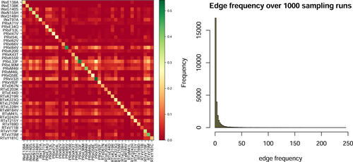
In the final step of the analysis we aim to collate the 1000 trees into a summarizing graph (a DAG) describing the evolution to resistance. For this purpose, we focus on the mutations, which are adjacent to the edges whose frequency is among the top 5-percentile in the summarizing ancestor matrix. The diagonal of the summarizing ancestor matrices show the fraction of how often the mutation is selected over all runs (Figure 1, left). PRxV32I is selected most often with a frequency of 0.541. Mostly, we find that for a pair of mutations, it does not happen frequently that each is the parent or ancestor of the other. The rows in the summarizing ancestor matrix with significantly high frequencies indicate mutations, for example, PRxI84V, which are mostly ancestors and almost never descendants of the same set of mutations.
Most mutations from our final set are already known to be mutations relevant for resistance to specific drug classes. This is not surprising since we used the Stanford Algorithm (version 9.1)10 and its set of resistance mutations with their respective scores to infer 4-CR labels. However, all previously independent classes or rather their respective mutations are put into context with each other in our evolutionary model. Furthermore, our set of 4-CR related mutations also includes mutations not used by the Stanford Algorithm to compute resistance, but known to be of accessory value to drug resistance. The mutations K55R, I66V and E34Q in protease (PR), V118I, E44D, E203K, K223Q, L228H, and Q242H in reverse transcriptase (RT) are not annotated as resistance mutation in the Stanford Algorithm. Margerison et al.23 identified K55R associated with M46I/L, which is in line with our evolutionary model that presents M46I as an ancestor and M46L as a descendant of K55R. I66V and E34Q have previously been identified as resistance mutations during PI treatment.24-27 Mutation V118I is known to be associated with resistance to the NRTI class.28 It also plays a part in dual resistance to AZT and 3TC together with mutation E44D.29 E203K has been identified as a contributor to emerging NRTI resistance and therapy failure.30-32 K223Q and L228H are less well investigated and more contextualized as accessory mutations,24, 33 while Q242H does not seem to be described at all. However, we observe Q242H on average in 12 of 250 genotypes, which makes it not less common than some well-known resistance mutations like E138A (12 of 250) and V82F (13 of 250). Q242H is also significantly associated with 4-CR according to our summarized tree and has the NRTI resistance mutation K219R as its parent.
2.2 POR
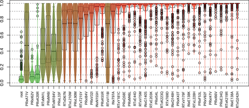
For each run we computed the POR of each mutation (Figure 2). In almost every run, some resistant genotypes did not contain any of the selected mutations. Hence, in general, we estimated a POR of greater than 0, around on average, for the root node, which depicts genotypes without any of the selected mutations. Even though we selected for mutations mostly observed in resistant genotypes, a mutation's POR can be low, indicating either a poor fit of the resistant genotypes to this position in the tree or a good fit of susceptible genotypes to the position. For example, if the mutation is a direct descendant of the root, an unmutated susceptible genotype fits with only one false negative, while resistant genotypes with more mutations fit relatively poorly due to false positives. More than half of all mutations show high POR. Mutations with high or low median POR show mostly low variance in their POR over all data sets. However, the closer the median to 0.5 the higher the variance. The distributions are mostly unimodal, but more or less uniform for the mutations PRxL33F and PRxA71V, which show a high variance of POR over all 1000 data sets. Hence, it depends very much on the context (other mutations, different tree), whether these mutations are indicators of high or low 4-CR.
2.3 Summarized evolutionary history
The directed graph defined by the adjacency matrix of edge frequencies (Figure 1) still includes cycles. For our summarized DAG model (history DAG), we selected edges the following way. In order from high-frequency to low-frequency taken from the summarizing ancestor matrix, we incrementally added edges to our graph, if the two mutations adjacent to the edge were contained in our set of selected mutations and if the edge did not create a (directed) cycle.
The resulting transitively reduced graph is depicted in Figure 3. In the figure, the frequency of an edge is depicted by its fatness. The history DAG can be transformed into a tree by only keeping the most frequent incoming (black) edge for each mutation (Figure 3). However, in this way, we would lose important information. For example, the edge PRxI62V PRxL33F has a relatively high frequency, but loses to the more frequent edge RTxM184V PRxL33F. However, the former edge gives evidence to the fact that genotypes acquiring the mutation PRxL33F often had acquired PRxI62V earlier.
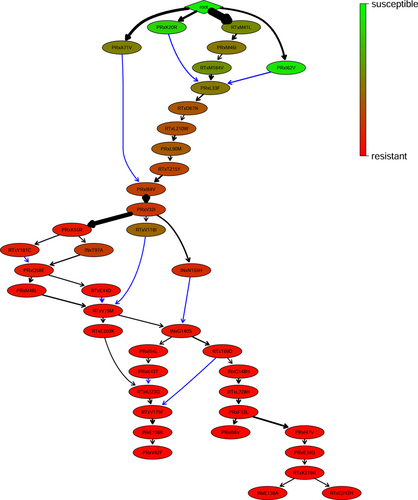
Many mutations close to the root also show low POR. The trend continues until around depth 11 (INxN155H, PRxK55R), when the mutations have a mean POR of over 90%. The violin boxplots (Figure 2) are sorted according to the increasing depth of the respective mutation in the history DAG. We observe that there is a monotonic increase in POR except for a few edges like PRxV32I RTxV118I.
Two edges are significantly more frequent than the others, root RTxM41L and PRxV32I PRxK55R. We will note that there are highly frequent edges that we can see in the summarizing ancestor matrix (Figure 1, left) but which are not included in the DAG (Figure 3) because that history DAG is a transitive reduction. One example of such an edge is the most frequent edge PRxL33F PRxV32I. Two interesting paths are those from the root to INxT97A and INxG140S, respectively. These paths include mutations from all three gene regions targeted by drugs and could explain the rise of 4-CR. Interestingly, we find only two mutations (RTxV179F, RTxY181C) associated with the NNRTI class in the Stanford Algorithm. However, these are known to be two of the most frequent mutations of the NNRTI drug class.34
Our history DAG implicitly also reflects the overall rather uniform history of therapies, which is aggregated over all genotypes. That is, mutations stemming from drugs inhibiting PR or RT arise earlier, while IN mutations appear later and indicate high resistance.
The history DAG helps us to interpret novel genotypes. For example, let us assume we observe a genotype with mutation V32I in PR. We can infer from the history DAG that we should also observe mutation L210W in RT, because we observed L210W in the ancestral viral strains of variants carrying V32I. If we do not observe L210W, the history DAG gives us two options. Option one is that V32I is a false positive, that is, we observe the mutation due to noise and it is actually not present in the virus. Option two is that L210W is a false negative, that is, the virus has the mutation, but we do not observe it, for example, due to noise or a back-mutation. The false negative rate is usually estimated greater than the false positive rate. The average estimated false positive and false negative rates over the 1000 data sets are 0.01 (SD: 0) and 0.26 (SD: 0.096), respectively. The average observed rates were similar with 0.02 (SD: 0.012) and 0.27 (SD: 0.085), respectively. However, these are the global rates over all mutations and we are also interested in mutation-specific error rates relating to our final evolutionary history. These error rates could give hints on hidden mutations of virus populations still present in the reservoir.
2.4 Mutation-specific error rates
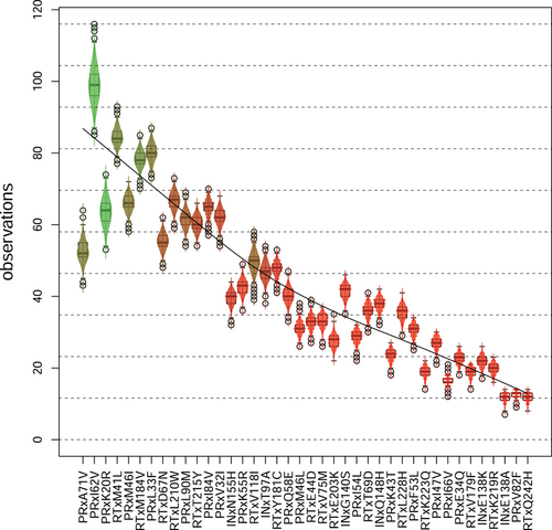
The resulting distributions for each mutation are highly dependent on its position in the history DAG (Figure 4). The false negative rate increases with the rising number of ancestors of a mutation. For example, if a mutation has no ancestors, the false negative rate is 0 by definition because no ancestors can be negative. Vice versa, the false positive rate is 0, if the mutation has no descendants. While 0 false negatives are practically only possible when a mutation has no ancestors and is at the top of the history DAG, mutations with false negatives are more evenly distributed along the graph. The false negative rate of a mutation is significantly greater than its false positive rate and has a higher variability for all mutations. In the left-hand panel of Figure 4, the false negative rate seems to reach a plateau roughly at the position of mutation K43T on the PR. This is confirmed by the total number of observations per mutation (Figure 5). The fewer observations the higher the false negative rate. The number of observations shows a similar but inverse trend, as its descent toward mutations with more ancestors gets flatter.
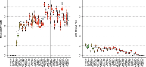
The high false negative rates imply a heavy loss of mutations in the visible genotype over time. However, it is possible that there is still virus harboring these mutations in the reservoir.11-13 While the variance of the false negative rate across all mutations is relatively large, its maximum is reached quite early along the history DAG, namely at G140S in IN with a false negative rate of roughly 0.52. Hence, we observe G140S while many of its ancestors are not observed. G140S is also associated with the Q148H pathway,35 which is expressed by our history DAG, because G140S is the grandparent of Q148H.
The false positive rate (Figure 4, right) also nicely correlates with the overall number of observations (Figure 5), that is, the more observations of a mutation, the higher the false positive rate. Interestingly, the number of observations of the first three mutations is anticorrelated with their false positive rate. For example, PRxI62V has the most observations but the lowest number of false positives of the three mutations.
3 DISCUSSION
We used the mathematical framework of mutagenetic trees to model the evolutionary accumulation of mutations in the context of four-class drug resistance. The mutagenetic history DAG elucidates mutations correlated with resistant and susceptible genotypes. Novel genotypes can be interpreted by placing them on the optimal position, the mutation representing the best-fitting genotype, in the history DAG. The graph imputes the full mutational profile of the genotype. For example, if the graph predicts a mutation that is not observed in the genotype, it could be that the mutation is lost in the currently dominating viral variant visible in blood serum, but still persistent in a virus kept in the tissue reservoir.
To our knowledge, this is the first time that accumulation of resistance is mathematically modeled across different drug classes and not exclusively within one drug class. Our model builds on methodology for inferring mutational history. However, this parametrization has not been used for mutagenetic trees before and provides the novel ability to compute a POR and a false positive and false negative rate specific to each mutation.
We confirmed many mutations already known as markers for resistance and identified novel mutations previously not in the focus of resistance analysis. We computed the POR for all significant mutations and their corresponding genotypes. Additionally, we computed error rates to identify mutations that imply subpopulations not visible in the blood serum but possibly still exist in the tissue reservoir. The information about hidden viral populations can be of vital importance for therapy treatment. A resistance-associated mutation in the hidden population can lead to a failing therapy. Such therapy failure increases the risk of formation of multidrug resistance. Knowledge about the patient's history derived from models such as our DAG can help to optimize therapy strategies and to increase the probability of therapy success.
Due to the complexity of the mutagenetic tree model, we cannot include all observed mutations at once. For each of overall 1000 subsampling runs we focused on 25 mutations to ensure that the optimal tree is found with high confidence. Hence, our final model of accumulation of mutations is a mixture of 1000 trees with 25 mutations each. This mixture corresponds to a DAG (history DAG) and does not abide to the simplified assumption of the tree anymore. For example, two parents correspond to two different lineages merging into a single one. However, the history DAG is still of practical use for the interpretation of mutational profiles.
Since multidrug resistance is not commonly considered, our data set consists of relatively few genotypes labeled as such. A larger number of 4-CR genotypes could make our evolutionary model more robust and interpretable. Especially, niche mutations, involved in multidrug resistance, are hard to find with low sample size.
Overall, our model, estimating the accumulation of mutations in the context of four-class drug resistance, can be helpful to interpret genotypes for potential resistance. However, there is still room for improvement. While our history DAG is driven by and reflects treatment history, it does not make any statements about individual drugs or therapies. It is not trivial to directly combine resistance level and mutations with drug exposure. Doing so could make the history DAG even more informative, especially if more 4-CR labeled genotypes were available.
4 METHODS
4.1 Definition of 4-class drug resistance
Resistance is computed by the Stanford Algorithm (version 9.1).10 The integer scores are binarized to 0 (score ) and 1 (score ).
-
Resistance to the NRTI class (abacavir [ABC], lamivudine [3TC], emtricitabine [FTC], tenofovir [TDF or TAF], zidovudine [AZT or ZDV])
-
Resistance to the NNRTI class (nevirapine [NVP], efavirenz [EFV], etravirine [ETR], rilpivirine [RPV], doravirine [DOR])
-
Resistance to the PI class (lopinavir [LPV], atazanavir [ATV], darunavir [DRV])
-
Resistance to the INSTI class (raltegravir [RAL], elvitegravir [EVG], dolutegravir [DTG], bictegravir [BIC])
4.2 Data preprocessing
We collect raw sequences from the EuResist Integrated Database (EIDB, version June 2022). Ethical approval was granted in the host countries of the respective original databases contributing data to EIDB. Sequences were aligned to the HXB2 reference genome. For the local alignment, we use a very efficient implementation of the Smith–Waterman algorithm, which was first developed by Eugen Schülter http://www.schuelter-gm.de/mutext.html, has been implemented as REST service by the geno2pheno team and is now used in the geno2pheno prediction server http://geno2pheno.org. We keep sequences with an aligned amino acid start position less or equal to 10 (PR), 41 (RT), 51 (IN), and stop position greater or equal to 90 (PR), 238 (RT), 232 (IN). The aligned genotypes are stored in a binary mutation matrix with each row a sequence and each column an amino acid position, and mutations defined as a change from the reference genome. For example, a mutation at position 55 in PR with the wild-type K changed to E is denoted by a 1 in the column PRxK55E.
4.3 Data filtering and subsampling
We select only full genotypes, that is, with PR, RT, and IN sequences. The genotypes are restricted to all observed mutations.
We reduce model complexity and account for the underlying model distribution and noise with a subsampling approach. First, we (uniformly) sample 90% of all genotypes annotated as four-class drug resistant. We balance the data set by adding the same amount of susceptible samples, which are not resistant to any drug. Second, we sample 25 of 6576 mutations with a probability for each mutation proportional to its frequency of occurrence in resistant genotypes. Let be the number of observations of mutation in resistant genotypes and the number of observations of the mutation in all genotypes. We compute the individual frequency by . We compute the share of mutation over all observations in resistant genotypes by . The overall selection probability is . Hence, we prefer mutations, which mostly () and often () occur in resistant genotypes.
The initial filtering for a full sequence (PR, RT, IN) leaves us with 125 resistant and 11 597 susceptible genotypes. For each sampled data set (1000 overall) we learn one tree with a heuristically maximized likelihood given the data.
The selection assures that we observed a high number of mutations (red) in resistant genotypes and a low number in susceptible genotypes (Figure 6). In the figure, resistant genotypes are indicated by the red ticks on top of the heatmap and susceptible genotypes by green ticks.

4.4 Mutagenetic tree
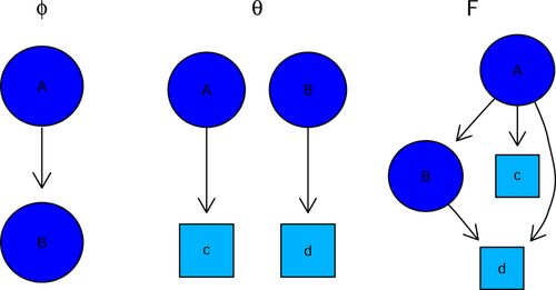
We use a slightly different model formulation of mutagenetic trees related to Tresch and Markowetz.18 We represent the transitive closure of a mutagenetic tree with mutations by an ancestor matrix with , if and only if mutation is an ancestor of mutation . The mutated genotypes and the mutations form a special subgraph represented by the matrix with , if and only if genotype is the child of mutation . We say genotype is attached to mutation , if . We assume that each genotype has at most one parent in . The predicted mutational profile for each genotype is computed by the matrix product . Hence, we should observe mutation and all ancestor mutations of in all genotypes attached to mutation . That is., if mutation is an ancestor of mutation () and genotype is the child of mutation (), we compute (see also toy example in Figure 7).
-
Prune and attach:
- –
Remove the edge with parent .
- –
Add the edge with new parent .
- –
-
Node flip: Swap the labels of nodes and in the tree.
-
Rate optimization: change (or ) by a given step size, for example, 0.01 with .
We avoid searching for an optimal attachment by computing the posterior . is set to 1, if and only if .
4.5 POR
Once an optimal tree has been learned, we can compute a POR for genotypes predicted by the tree. The known resistance of the observed genotypes is stored in a binary vector with , if genotype is resistant and otherwise. The resistance of predicted genotypes is denoted by .
4.6 Mutation-specific error rates
We compute error rates for each mutation based on our summarized model. However, we eliminate the tree assumption and base our computations on the dag structure including blue edges.
AUTHOR CONTRIBUTIONS
Martin Pirkl, Anders Sönnerborg, Francesca Incardona, Anne-Mieke Vandamme, Maurizio Zazzi, Rolf Kaiser, and Thomas Lengauer conceptualized the study. Carole Devaux, Michael Böhm, Anders Sönnerborg, Francesca Incardona, Ana Abecasis, Anne-Mieke Vandamme, and Maurizio Zazzi managed data curation and access. Martin Pirkl and Joachim Büch processed the data. Martin Pirkl conducted the statistical analysis under supervision of Thomas Lengauer. Martin Pirkl, Rolf Kaiser, and Thomas Lengauer interpreted the results. Martin Pirkl, Rolf Kaiser, and Thomas Lengauer wrote the initial draft of the manuscript. All authors have read and agreed to the published version of the manuscript.
ACKNOWLEDGMENT
This study was partially funded by ViiV Healthcare. The authors are solely responsible for final content and interpretation.
ETHICS STATEMENT
Ethical approval was granted in the host countries of the respective original databases contributing data to EIDB.
Open Research
DATA AVAILABILITY STATEMENT
Restrictions apply to the availability of these data. Data were obtained from the EuResist Network and are available for request through a study application form at https://www.euresist.org/become-a-partner with the permission of the EuResist Network.


